Financial development
A natural way in which the expansion of the variety of industries can generate complementarities in the growth process is through its effects on financial markets. Acemoglu and Zilibotti (1997) construct a model where the introduction of new securities, associated with the development of new intermediate industries, improves the diversification opportunities available to investors.
Investors react by supplying more funds, which fosters further industrial and financial development, generating a feedback.[65] The model offers a theory of development. At early stages of development, a limited number of intermediate industries are active (due to technological nonconvexities), which limits the degree of risk-spreading that the economy can achieve. To avoid highly risky investments, agents choose inferior but safer technologies. The inability to diversify idiosyncratic risks introduces a large amount of uncertainty in the growth process. In equilibrium, development proceeds in stages. First, there is a period of “primitive accumulation” with a highly variable output, followed by take-off and financial deepening and finally, steady growth. Multiple equilibria and poverty traps are possible in a generalized version of the model.The theory can explain why the growth process is both slow and highly volatile at early stages of development, and stabilizes as an economy grows richer. Evidence of this pattern can be found in the accounts of pre-industrial growth given by a number of historians, such as Braudel (1979), North and Thomas (1973) and De Vries (1990). For instance, in cities such as Florence, Genoa and Amsterdam, prolonged periods of prosperity and growth have come to an end after episodes of financial crises. Interestingly, these large set-backs were not followed (as a neoclassical growth model would instead predict) by a fast recovery but, rather, by long periods of stagnation.
Similar phenomena are observed in the contemporary world. Acemoglu and Zilibotti (1997) document robust evidence of increases in GDP per capita being associated with large decreases in the volatility of the growth process. It has also been documented that higher volatility in GDP is associated with lower growth [Ramey and Ramey (1995)].We here describe a simplified version of the model. Time is discrete. The economy is populated by overlapping generations of two-period lived households. The population is constant, and each cohort has a mass equal to L. There is uncertainty in the economy, which we represent by a continuum of equally likely states s ∈ [0, 1]. Agents are assumed to consume only in the second period of their lives.[66] Their preferences are parameterized by the following (expected) utility function, inducing unit relative risk
aversion:

The production side of the economy consists of a unique final good sector, and a continuum of intermediate industries. The final good sector uses intermediate inputs and labor to produce final output. Output in state s ∈ [0, 1] is given by the following production function:

For simplicity, we assume L = 1. The term in brackets is “capital”, and it is either produced by a continuum of intermediate industries, each producing some state-contingent amount of output (χs), or a separate sector using a “safe technology” (χφ). The measure of the industries with a state-contingent production, At, is determined in equilibrium, and At can expand over time, like in Romer’s model, but it can also fall. Moreover, At ∈ [0, 1], i.e., the set of inputs is bounded.
In their youth, agents work in the final sector and earn a competitive wage, wsφ = (1 - α)Ysφ.Atthe end of this period, they take portfolio decisions: they can place their savings in a set of risky securities ({Fi }i∈[0 At]), consisting of state-contingent claims to the output of the intermediate industries or, in a safe asset (φ), consisting of claims to the output of the safe technology.
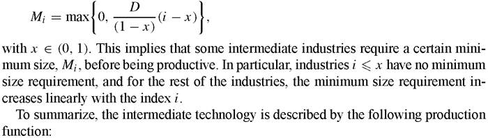
After the investment decisions, the uncertainty unravels, the security yields its return and the amount of capital brought forward to the next period is determined. The capital is then sold to final sector firms and fully depreciates after use. Old agents consume their capital income and die.Intermediate industries use final output for production. An intermediate industry i ∈ [0, At ] is assumed to produce a positive output only if state s = i occurs. In all other states of nature, the firm is not productive. Moreover, the ith industry is only productive if it uses a minimum amount of final output, Mi, where
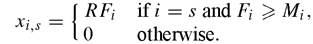
Since there are no start-up costs, all markets are competitive. Thus, firms retain no profits, and the product is entirely distributed to the holders of the securities. The jth security entitles its owner to a claim to R units of capital in state j (as long as the minimum size constraint is satisfied, which is always the case in equilibrium), and otherwise
F(A)
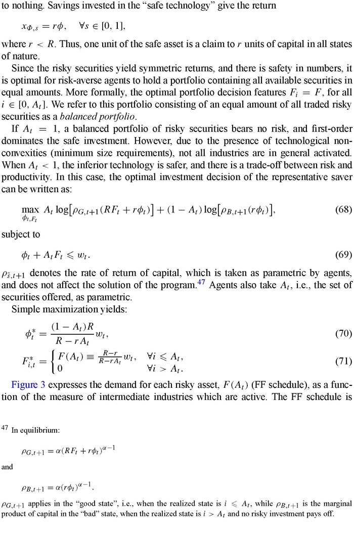
Figure 3.
upward sloping, implying that there is complementarity in the demand for risky assets: the demand for each asset grows with the variety of intermediate industries.
Complementarity arises because the more active are intermediate industries, the better is risk-diversification. Thus, as At increases, savers shift their investments away of the safe asset into high-productivity risky projects (the “stock market”). Such complementarity hinges on risk aversion being sufficiently high.48 In general, similar to Young (1993), an increase in A creates two effects.
On the one hand, investments in the stock market become safer because of better diversification opportunities, which induces complementarity. On the other hand, investments are spread over a larger number of assets, inducing substitution. With sufficiently high risk aversion, including the unit CRRA specification upon which we focus, the first effect dominates.The equilibrium measure of active industries, A*, is determined (as long as A* < 1) by the following condition: 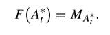
[1] Suppose agents were risk averse, but only moderately so. Suppose, in particular, that they were so little risk-averse that they would decide not to hold any safe asset in their portfolio. Then, an expansion in the set of risky securities would induce agents to spread their savings (whose total amount is predetermined) over a larger number of assets. In this case, assets would be substitutes rather than complements.
In Figure 3, the equilibrium is given by the intersection of schedules FF and MM, where the latter represents the distribution of minimum size requirements across industries. Intuitively, A* is the largest number of industries for which the technological non-convexity can be overcome, subject to the demand of securities being given by (71).49
Growth increases wage income and the stock of savings over time. In equilibrium, this induces an expansion of the intermediate industries, A*. This can once more be seen in Figure 3: growth creates an upward shift of the FF schedule, causing the equilibrium to move to the left. Therefore, growth triggers financial development. Inparticular, when the stock of savings becomes sufficiently large, the financial market is sufficiently thick to allow all industries to be active. In the case described by the dashed curve, FF', the economy is sufficiently rich to afford A* = 1. The inferior safe technology is then abandoned.
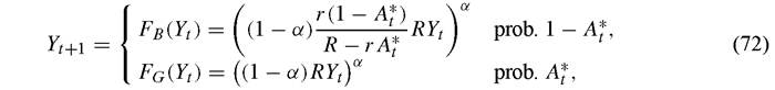
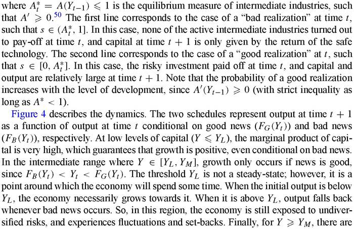
Financial development, speeds up growth by channelling investments towards the more productive technology.The stochastic equilibrium dynamics of GDP can be explicitly derived: [67]
[1] Acemoglu and Zilibotti (1997) show the laissez-faire portfolio investment to be inefficient. Efficiency would require more funds to be directed to industries with large non-convexities, i.e., agents not holding a balanced portfolio. The inefficiency is robust to the introduction of a rich set of financial institutions.
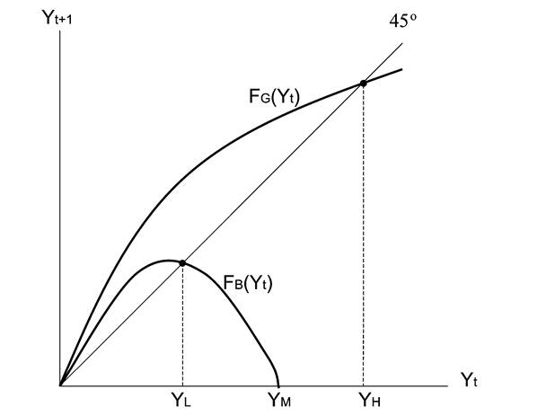
Figure 4.
enough savings in the economy to overcome all technological non-convexities. When the economy enters this region, all idiosyncratic risks are removed, and the economy deterministically converges to Yh.[68]
Note that it may appear as if, in the initial stage, countries striving to take off do not grow at a sustained rate during long periods. The demand for insurance takes the form of investments in low-productivity technologies, and poor economies tend to have low total factor productivity and slow growth.
In the case described by Figure 4, the economies “almost surely” converge to a unique steady-state. Different specifications of the model can, however, lead to less optimistic predictions. With higher risk aversion, for instance, traps can emerge, as in the example described in Figure 5. An economy starting with a GDP in the region [0, Ymm) would never attain the high steady-state Yh, and would instead perpetually wander in the trapping region [0, Yll]. Conversely, an economy starting above Ym would certainly converge to the high steady-state, Yh. Finally, the long-run fate of an economy starting in the region [Ymm, Ym ] would be determined by luck: an initial set of positive
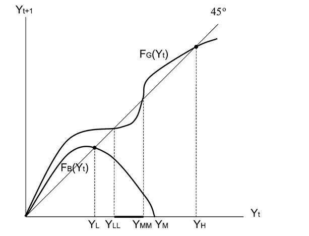
Figure 5.
draws would bring this economy into the basin of attraction of the good equilibrium. A single set-back, however, would forever jeopardize its fιιture development.[69]
The model can be extended in a number of directions. A two-country extension shows that international capital flows may lead to divergence, rather than convergence between economies. This result is due to the interplay between two forces: first, decreasing returns to capital would tend to direct foreign investments towards poorer countries, as in standard neoclassical models. Second, the desire to achieve better diversification pushes investments towards thicker markets. The latter force tends to prevail at some earlier stages of the development process. So, poor countries suffer an outflow of capital, which spills over to lower income and wages for the next generation, thereby slowing down the growth process. The analysis of capital flows, financial integration and financial crises in the context of similar models is f'urther developed in recent papers by Martin and Rey (2000, 2001 and 2002). A different extension of the model is pursued by Cetorelli (2002) who shows that the theory can account for phenomena such as “club convergence”, economic miracles, growth disasters and reversals of fortune.
Recent empirical studies analyze implications of the theory about the patterns of risk-sharing and diversification. Kalemli-Ozcan et al. (2001, 2003) document that regions with access to better insurance through capital markets can afford a higher degree of specialization. Using cross-country data at different levels of disaggregation, Imbs and Wacziarg (2003) find robust evidence of sectoral diversification increasing in GDP However, their findings also suggest that, at a relatively late stage of the development process, the pattern reverts and countries once more start to specialize. This tendency for advanced countries to become more specialized as they grow can be explained by factors emphasized by the “new economic geography” literature [Krugman (1991)], from which the theory described in this section abstracts, such as agglomeration externalities and falling transportation costs.
7.
More on the topic Financial development:
- Alsharari Nizar Mohammad (ed.). Banking and Accounting Issues. ITexLi,2022. — 175 p., 2022
- Acknowledgments
- Dynamic equations
- Hare C., Neo D. (eds.). Trade Finance: Technology, Innovation and Documentary Credit. Oxford University Press,2021. — 417 p., 2021
- Foreword: Frances Moore Lappe
- AAP. Guidelines for Air and Ground Transport of Neonatal and Pediatric Patients. 4th edition. — American Academy of Pediatrics,2015. — 488 p., 2015
- Malta
- An evolutionary analysis of multilevel governance mechanisms for SHD at the local level
- Zimbabwe Village Savings and Loan Associations