Endogenous volatility and amplified shocks

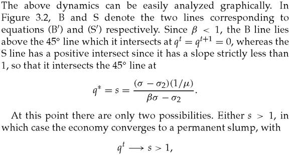
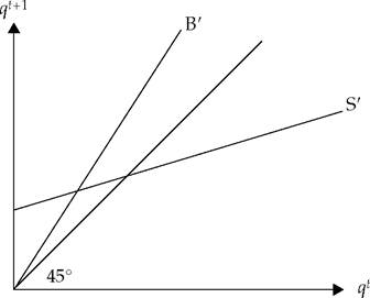
Fig.

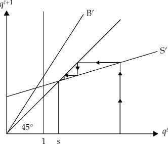
Fig. 3.3 The permanent slump regime.

so that indeed investment demand is always less than total savings for t sufficiently large. This case is depicted in Figure 3.3. Or s < 1, in which case the economy will converge to a limit cycle, as shown in Figure 3.4, oscillating between boom and slump phases.

The intuition for these cycles can be simply summarized as fol­lows. Starting from a slump phase, investments and borrowing will resume growing over time as entrepreneurs are getting richer, and eventually, investment capacity μWB will run ahead of sav­ings. At this point, savings will be fully employed in the high-yield

Fig. 3.4 The cycles regime.

technology which means that the economy will grow fast at rate g, but the interest rate will also rise up to σ1 = βσ. This rise in interest rate will increase the debt burden of all entrepreneurs (this is the pecuniary externality part of the story). The rise in the debt burden will slow down the growth of entrepreneurs' wealth and therefore that of their investment capacity (this is the credit con­straint part of the story) relative to that of total savings, so that at some point investment capacity will fall below total savings, at which point the economy will enter a slump phase and the interest rate will fall to σ2. The economy will then grow at a rate lower than g, however, the low interest rate will allow entrepreneurs to rebuild their investment capacity so as to eventually absorb all aggregate savings, at this point the economy will reenter a boom, and so on.

Two remarks are worth making at this point:

1. Note that the economy may stay for several periods in a row in one regime (either boom or slump) before switching to the other regime, as shown in Figures 3.5 and 3.6.

2. Persistent limit cycles occur when

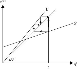
Fig. 3.5 Prolonged boom (debt buildup).

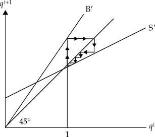
Fig. 3.6 Prolonged recession (profit reconstitution).

or equivalently when

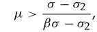
that is for sufficiently high levels of financial development as measured by the credit multiplier μ. In particular, a highly underdeveloped economy in which entrepreneurs rely entirely on their retained earnings for investment (that is, where μ = 1) will not cycle. On the other hand, an economy where firms face no credit constraint and can invest up to the expected net present value of their projects, will not experience long-term volatility either, as

in that case. It is thus only those economies at intermediate levels of financial development which will experience per­sistent fluctuations. Thus, the model provides an explanation for why we tend to observe more volatility in middle-income countries in Asia or Latin America than either in highly developed countries like the United States or the highly underdeveloped countries of Africa.

Finally, let us analyze what exogenous productivity shocks do in this model, keeping in mind the usual criticism of the RBC literature that it is unable to explain the magnitude of observed fluctuations. More specifically, consider the effect of a temporary shock that increases the productivity parameter σ, and suppose that prior to this shock the economy is at the steady-state q^t = s.

From equation (S'), we immediately see that the positive shock on σ shifts the S curve as shown in Figure 3.7, toward a modified

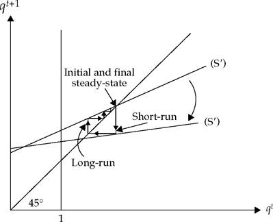
Fig. 3.7 Effect of temporary increase in σ.

Source: Aghion et al. (1999a), figure IXa.

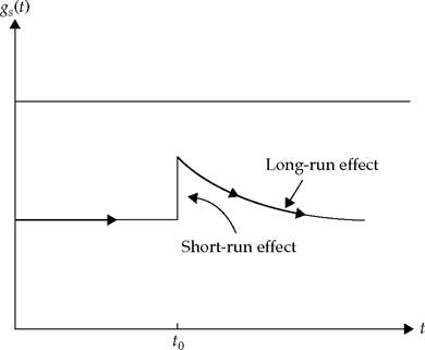
Fig. 3.8 Effect of temporary increase in σ on growth. Source: Aghion et al. (1999a), figure IXb.

curve with lower slope and higher intercept. As a result, q^t falls before moving back up monotonically toward its initial value.

The growth rate equal to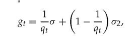

will then evolve as shown in Figure 3.8, first increasing sharply and then going back slowly to its initial level. We thus see that the direct effect of the productivity shock on the growth rate (dir­ect effect of σ on g_t) is amplified by the indirect effect through q_t: namely, a positive productivity shock increases entrepreneurs' wealth and therefore their borrowing capacity. This in turn allows them to absorb a higher fraction of aggregate savings into their high-yield production technology, which itself operates at (tem­porarily) higher productivity. The persistence is due to the fact that entrepreneurs' borrowing capacity is positively affected not only in the short run, but also after productivity has returned to its initial level, as entrepreneurs can carry their wealth from one period to the next.⁶

^[I] This amplifying mechanism is essentially that pointed out by BG, although here it is analyzed in the context of a fully dynamic general equilibrium model.

3.5