Models with common growth driven by international knowledge spillovers
Based on evidence in the previous section, we now focus on models with two features. The first is that, in steady state, all countries grow at the same rate thanks to international knowledge spillovers.
The second feature is that differences in policies or other country parameters generate differences in TFP levels rather than growth rates. Examples of this type of model are Howitt (2000), Parente and Prescott (1994), and Eaton and Kortum (1996, 1999), as well as the model of technology diffusion in Chapter 8 of Barro and Sala-i-Martin (1995). Eaton and Kortum (1999) is a particularly close predecessor to our approach, although they go farther in tying their analysis to international patenting data in the G5 countries.In these models there is a world technology frontier, and a country’s research efforts determine how close the country gets to that frontier. There are three different issues that must be addressed. First, what determines the growth rate of the world technology frontier? Second, how is it that a country’s research efforts allow it to “tap into” the world technology frontier? And third, what explains differences across countries in their research efforts? Our goal in this section is to build on the ideas developed in the recent literature to construct a model that offers a unified treatment of these three issues and that is amenable to calibration. The calibration is intended to gauge the model’s implications about the strength of the different externalities and the drivers of cross-country productivity differences.[506]
To highlight the different issues relevant for the model, our strategy is to present it in parts. The next subsection 4.1 takes world growth and R&D investment as exogenous and discusses how R&D investment determines steady state relative productivity. Subsection 4.2 discusses different ways of modeling how world-wide R&D investment determines the growth rate of the world technology frontier.
Subsection 4.3 extends the model so as to allow for endogenous determination of countries’ R&D investment rates. Subsection 4.4 calibrates the model. Finally, subsection 4.5 presents the results of an exercise where we calculate, for each country in our sample, the impact on productivity from international spillovers.4.1. R&D investment and relative productivity
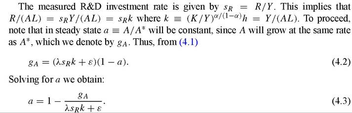
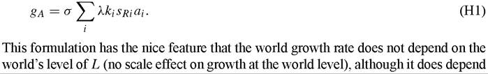
In this section we focus on a single country whose research efforts determine its productivity relative to the world technology frontier. Both the R&D investment rate and the rate of growth of the world technology frontier are exogenous. Output is produced with a Cobb-Douglas production function: Y = Kα(AhL)1~α,where Y is total output, K is the physical capital stock, A is a technology index, h is human capital per person, and L is the total labor force. We assume that h is constant and exogenous. Output can be used for consumption (C), investment (I), or research (R), Y = C + pI + R, where p is the relative price of investment and is assumed constant through time. Capital is accumulated according to: K = I — δK. Finally, A evolves according to:

where λ is a positive parameter and A* is the world technology frontier, both common across countries.[507]
There are three salient differences between this model and the standard endogenous growth model. Firstly, the productivity of research in generating A-growth is affected by the country’s productivity relative to the frontier, as determined by the term (1 - A/A*) in (4.1). This captures the idea that there are “benefits to backwardness”. One reason for this may be that the effective cost of innovation and technology adoption falls when a country is further away from the world technology frontier. This is what happens in Parente and Prescott (1994) and in Barro and Sala-i-Martin (1995, Chapter 8).
Alternatively, being further behind the frontier may confer an advantage because every successful technology adoption entails a greater improvement in the national technology level. This is what happens in Howitt (2000) and in Eaton and Kortum (1996).9Secondly, we introduce ε f 0 to capture the sources of technology diffusion from abroad that do not depend on domestic research efforts. We have in mind imports of goods that embody technology, and that do not require upfront adoption costs (e.g., equipment which is no harder to use but which operates more efficiently).10 As we will see below, this is important for the model to match certain features of the data.
Thirdly, in contrast to most endogenous growth models, we divide research effort by L in the A -growth expression above. This is done to get rid of scale effects and can be motivated in two ways. First, if A represents the quality of inputs, then one can envisage a process where an increase in the labor force leads to an expansion in the variety of inputs [Young (1998) and Howitt (1999)]. Withalargervariety of inputs, research effort per variety is diluted. This eliminates the impact of L on A growth. Second, if research is undertaken by firms to increase their own productivity, then population growth may lead to an expansion in the number of firms and a decrease in the impact of aggregate research on firms’ A-growth [Parente and Prescott (1994)]. In this case, L represents the number of firms.
The values of k and sR determine a country’s relative A from (4.3). Conceivably, the parameter λ (TFP in research, if you will) could differ across countries and also contribute to differences in A. But in this paper we assume λ does not vary across countries. We 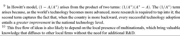
do, however, allow researchers to be more productive in countries with more physical and human capital per worker.
The previous results clearly show that policies that lower investment in physical or human capital or R&D do not affect a country’s growth rate. Their effect is on a country’s steady state relative A. Also, as discussed above, there are no scale effects in this model: higher L does not lead to higher growth or to a higher relative A. This stands in contrast to most growth models based on research [e.g., Romer (1990), Barro and Sala-i-Martin (1995, Chapter 8)].
It is also noteworthy in Equation (4.3) that the value of k, which captures physical and human capital intensity, affects a country’s TFP level conditional on its R&D investment rate. Thus, large differences in TFP across countries do not necessarily imply that differences in human and physical capital stocks are just a small part of cross country income differences. Indeed, this model suggests that some of the TFP differences may be due to differences in capital intensities across countries. Below we explore this issue quantitatively.
It is instructive to calculate the social rate of return to research at the national level. As shown in Jones and Williams (1998), this can be done even without knowing the details of the model that affect the endogenous determination of the R&D investment rate. Letting A = G(A, R), Jones and Williams show that the (within-country) social rate of return r can be expressed as:

(4.4)
Here Pa stands for the price of ideas and is given by Pa = (∂G∕∂R)-1. As explained by Jones and Williams, the first two terms in (4.4) represent the dividends of research while the third term represents the associated capital gains. The first dividend term is the obvious component, namely the productivity gain from an additional idea divided by the price of ideas. The second dividend term captures how an additional idea affects the productivity of future R&D.
In the model we presented above, it is straightforward to show that, along a steady state path, we have:

The first term on the right-hand side corresponds to the first dividend term in Jones and Williams’ formula. The second term, in square brackets, corresponds to the indirect effect of increasing A on the cost of research (∂G∕∂A). The third term, gL, corresponds to the term capturing the capital gains in Jones and Williams formula. To understand this last term, note that we have implicitly assumed that new varieties or firms start up with the same productivity as existing varieties or firms. Thus, the value of ideas will rise faster with a higher gL, and the social return to research will correspondingly increase with gL.
4.2. Modeling growth in the world technology frontier
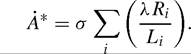
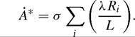
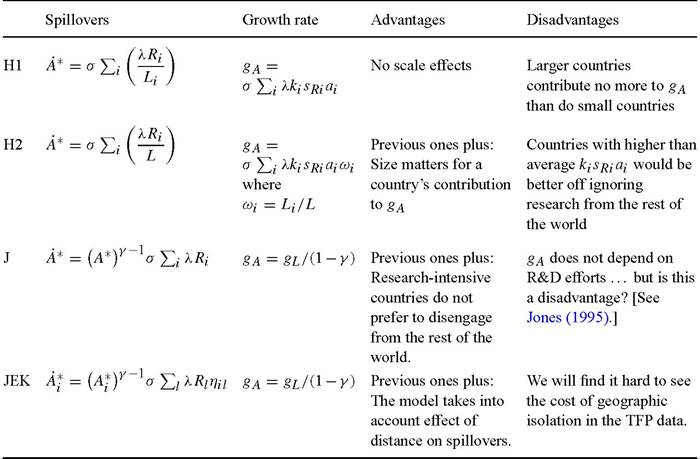
In this section we extend the model so that gA is endogenously determined by the research efforts in all countries. The models we mentioned above deal with this in different ways, except Parente and Prescott who leave gA as exogenous. Barro and Sala-i-Martin (1995, Chapter 8) have a Romer-type model of innovation that determines gA in the “North”. We do not pursue this possibility because of the scale effect that arises in their model (larger L in the North leads to higher gA) and because we want to allow research efforts by all countries to contribute to the world growth rate. We first consider an adaptation of Howitt’s (2000) formulation. A country’s total effective research effort, λRi, gets diluted by the country’s number of varieties or number of firms, both represented by Li, and is then multiplied by a common spillover parameter, σ, to determine that country’s contribution to the growth of the world’s technology frontier:
Given our results above, we obtain:
[1] The problem is not so pronounced forthe U.S.
Given its measured R&D investment rate of sr = 2.5%, we have r ≈ 40%, which is in the range of estimates of the social rate of return to R&D in the U.S. See Griliches (1992) and Hall (1996).positively on R&D investment rates. The main problem with this formulation, and the reason we do not pursue it further, is that larger countries contribute no more to world growth than smaller countries do. This has the implausible implication that subdividing countries would raise the world growth rate.
In footnote 22 of his paper, Howitt discusses an alternative specification wherein country spillovers are diluted by world variety rather than each country’s variety. This implies that:
where L = ∑ Li. Howitt does not pursue this approach because, in the presence of steady-state differences in the rate of growth of L across countries, gA would be completely determined in the limit by the research effort of the country with the largest rate of growth of L. We believe, however, that it is quite natural to analyze the case in which gL is the same across countries.[508] In this case, ωi ? Li /L is constant through time, and the expression above can be manipulated to yield:

If we think of L as the number of firms rather than the number of varieties of capital goods, then (H2) amounts to stating that gA is determined by the country-workforce- weighted average research intensity across firms world-wide. This seems much more reasonable than (H1), where gA is determined by the unweighted average of research intensity across countries.
Expression (H2) differs from (H1) only in the presence of the weights ωi that represent shares of world L. This has two advantages: first, large countries contribute more to world growth than small countries do, and second, subdividing countries would not affect the world growth rate. But (H2) has a problematic implication, namely that those countries with higher than average kisRi ai would be better off disengaging from the rest of the world - their growth rate would be higher if they were isolated. That is, a research intensive country would be better off ignoring the research done in other countries.
According to Howitt’s variety interpretation of this model, this is because an isolated country’s growth rate would be given by σλkisRiai. Its research intensity would no longer be spread out over the number of world varieties, but instead over the smaller number of the country’s own varieties. Thus, when a country disengages, it no longer benefits from spillovers from research conducted by the rest of the world, but there is an important compensating gain that comes from the fact that variety - and therefore dilution - falls for the disengaging country. Since there is no love of variety in Howitt’s model, a high research-intensity country would gain from disengagement. By this logic, engagement could not be sustained among any set of asymmetric countries! The higher klsκιal countries would always prefer to disengage, leaving all countries isolated in equilibrium.
We now turn to an alternative specification for world spillovers in which variety does not play such a crucial role. The specification will exhibit several of the features we have been looking for: first, no scale effect of world population on the world’s growth rate; second, other things equal, larger countries contribute more to world prosperity than small countries do; and third, tapping into rest-of-world research does not require spreading research across more varieties. We believe this is accomplished by adopting the formulation in Jones (1995): instead of dividing by L, the scale effect is avoided by introducing the assumption that advancing the world technology frontier gets harder as the frontier gets higher. This can be captured by the following specification of international spillovers:
where γ < 1. In this setting, sustained growth in A* depends on a continuously rising population. To see this, notice that we can restate (4.6) as follows:
)
l
This expression makes clear that gA is decreasing in A*; as mentioned above, this is what is going to eliminate the scale effect. Since all of the terms in the summation on the right-hand side of (J) are constant, then - differentiating with respect to time - we get that:

One criticism of this specification is that gA does not depend on sR, hence policy- induced increases in research intensity would not increase the world’s growth rate [Howitt (1999)]. As Jones (2002) argues, however, research intensity has been increasing over the last decades without a concomitant increase in the growth rate, so it is far from clear that we want a model where gA depends on sR.[509]
An interesting and relevant feature of the model presented by Eaton and Kortum (1996) is that it allows for spillovers to differ between pairs of countries. We can introduce this feature in the model by doing two things: first, we allow each country to

Table 6
Alternative ways of modeling international spillovers
14 If one takes F = 1 literally, then the externalities are in the human capital investment of individual workers.
15 We should note here that the tax rate on capital income also affects the incentive to do research. The notation used for the two tax rates is meant to emphasize that τκi affects all forms of accumulation by the firm, whereas TRi only affects research expenditures.
16 We assume that any tax revenue collected is distributed back to consumers in lump-sum fashion.
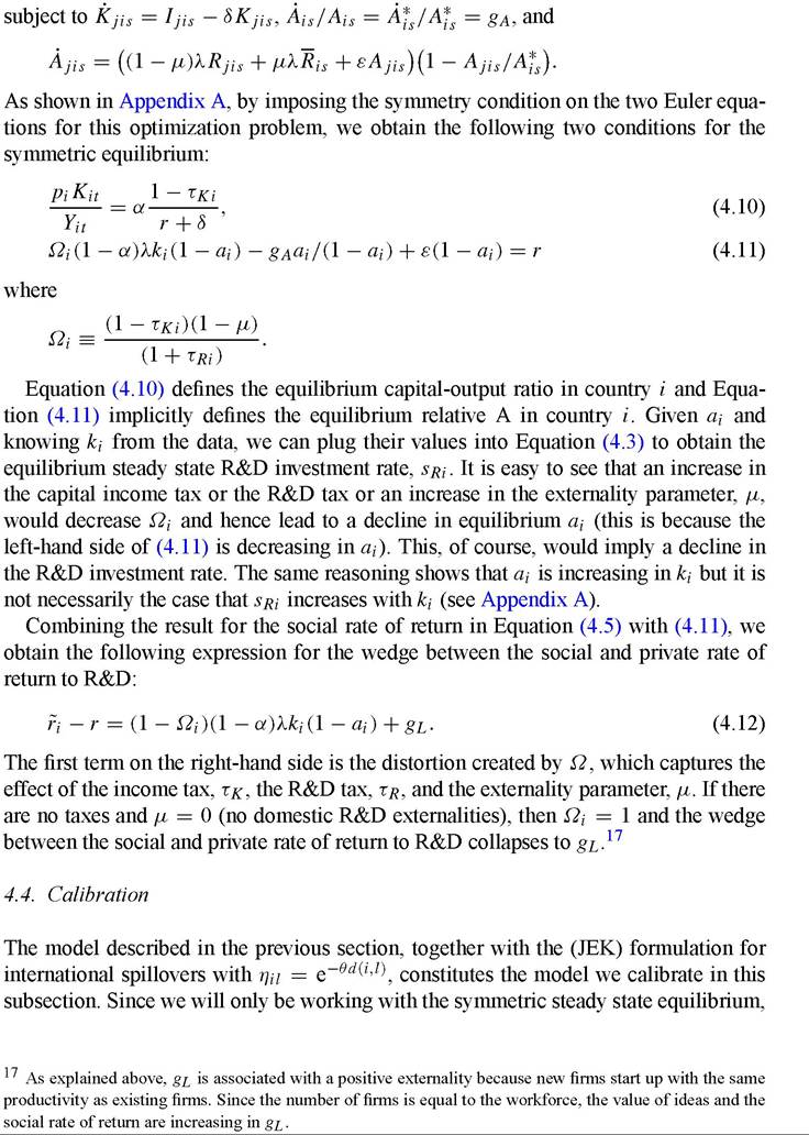
in this subsection we suppress time and firm subscripts to simplify notation. Given N countries, the steady state equilibrium is given by {Ki, Yi, ki, ai, sRi, Ai, A*, zi; i = 1,..., N} such that:
where the last equation comes from (JEK) together with (4.8).
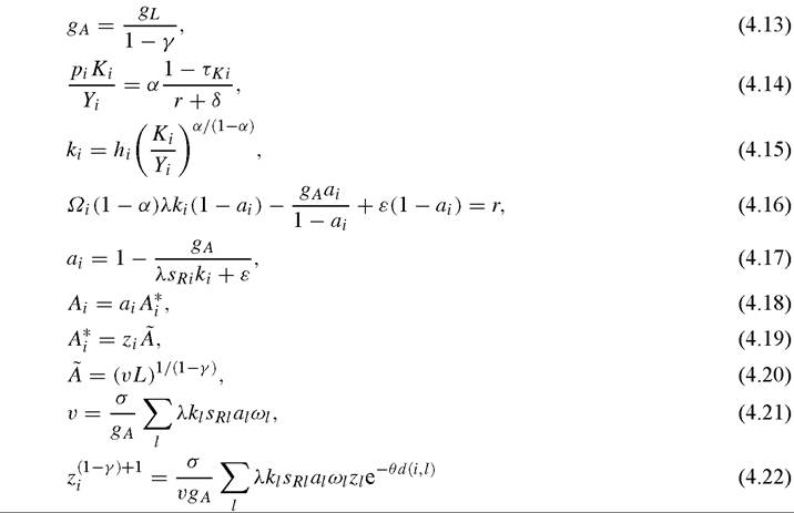
If we knew the relevant parameters and tax rates and wanted to solve for an equilibrium, we would first start by solving for gA from Equation (4.13). Given data for exogenous variables hi, pi and rKi we could then calculate equilibrium ki using (4.14) and (4.15). Together with gA and parameter ε, Equation (4.16) would yield ai. From (4.17) we would then obtain sRi. Up to this point, there is no interaction across countries, so these results do not depend on geography or θ; this dimension becomes relevant in obtaining actual productivity levels, because they depend on the variables zi, which capture spillovers from the rest of the world to country i. To see how this operates, note that given the value of θ, Equation (4.22) configures a system of N equations (where N is the number of countries) in N unknowns (z1, z2,...,zn ). The solution to this system determines zi. Given parameter σ, Equation (4.20) determines A, which together with zi determines each country’s technology frontier A* (Equation (4.19)). Finally, from Equation (4.18), a country’s technology frontier together with its relative A level ai determines Ai.
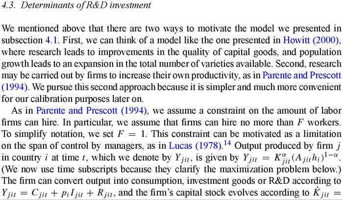
For the calibration exercise, the first step is to specify the variables we observe and how they relate to the model. We take human capital to be hi = eψ MYSi, where MYSi is mean years of schooling of the adult population in country i, obtained from Barro and Lee (2000). We use R&D data from Lederman and Saenz (2003). The 48 countries in our sample are the ones for which there is R&D data for 1995, as well as the necessary TFP and capital intensity variables described in Section 3. The first two columns of Table 7 reproduce the values of the R&D investment rate and the value of A for the 48 countries in our sample.
Forthebasicparametersweusethefollowingvalues: φ = 0.085, α = 1/3, S = 0.08, gL = 0.011 and gA = 0.015. For the first three, see our discussion in Section 3. The last two (the growth rates) were obtained from OECD average growth rates of L and A for the period 1960-2000.[510] Using (4.13), the values for the two growth rates imply γ = 0.31. To calculate the net private rate of return, r, which we assume to be common across countries, we take the capital income tax in the U.S. to be 25% (rκ,US = 0.25).[511] Given the 1995 U.S. nominal capital-output ratio of 1.5 (see Section 3 for how we constructed capital-output ratios), this implies from (4.14) that r = 8.6%. Given this level for r, we then use Equation (4.14) together with country nominal capital-output ratios to obtain each country’s implicit income tax τκi.
Remainingparameterswemustcalibrateare ε, λ, μ and θ. Unfortunately, there is no empirical work that we can rely on to pin down ε. Thus, we choose a value for ε based on the following reasoning. First, ε cannot be much higher than gA. This is because for ksR '≥ 0 Equation (4.17) implies that a '≥ 1 -gA∕ε. Thus, a high value of ε would imply that some countries’ relative empirical A becomes lower than the theoretical minimum 1 - gA∕ε. In other words, if free technology diffusion is too important, then it would be hard to account for countries with very low A levels. Second, if ε < gA, then countries with a low value of ksR (ksRk < gA - ε) would not be able to keep up with the world’s rate of growth in technology, so they would not have a steady state relative A level. (Consistent with stable long run relative income levels, Figure 3 showed roughly parallel slopes for average income across deciles over 1960-2000, with each decile based on 1960 income.) Thus, it seems reasonable to impose the intermediate condition that ε = gA. We believe, however, that future empirical work should attempt to understand the importance of free technology diffusion captured by parameter ε.
Given this choice for ε, we use two empirical findings to pin down parameters λ and μ, namely that the social rate of return to R&D in the U.S. is three times the net private rate of return [Griliches (1992)] and that the U.S. imposes a subsidy of 20% on R&D [Hall and Van Reenen (2000)], implying that Trus = -0.2.[512] Given data for sR and k for the U.S. in 1995 (srus = 2.5% and kUS = 3.6), then this restriction together with Equation (4.17) implies aUS = 0.7 and λ = 0.38.[513] From (4.16) we then obtain μ = 0.55.
Table 7
Data and “true” values for research intensity and productivity
| Country | Data sr | Data A | “True” Sr | Implied A |
| Argentina | 0.41% | 9,720 | 1.21% | 9,719 |
| Bolivia | 0.37% | 4,672 | 0.74% | 4,672 |
| Brazil | 0.86% | 9,836 | 1.67% | 9,835 |
| Chile | 0.61% | 11,078 | 1.98% | 11,075 |
| China | 0.60% | 2,570 | 0.28% | 2,570 |
| Colombia | 0.28% | 8,143 | 1.54% | 8,141 |
| Ecuador | 0.08% | 5,990 | 0.69% | 5,990 |
| Egypt | 2.11% | 11,126 | 3.57% | 11,119 |
| Hong Kong | 0.25% | 17,874 | 5.49% | 17,732 |
| Hungary | 0.73% | 7,172 | 0.63% | 7,172 |
| Indonesia | 0.09% | 5,912 | 0.91% | 5,911 |
| India | 0.63% | 3,755 | 0.60% | 3,755 |
| Israel | 2.75% | 13,919 | 2.15% | 13,922 |
| South Korea | 2.49% | 8,842 | 0.71% | 8,843 |
| Mexico | 0.31% | 8,781 | 1.08% | 8,780 |
| Panama | 0.38% | 6,106 | 0.60% | 6,106 |
| Peru | 0.05% | 4,285 | 0.40% | 4,285 |
| Poland | 0.69% | 4,893 | 0.33% | 4,893 |
| Romania | 0.80% | 2,757 | 0.16% | 2,757 |
| Senegal | 0.02% | 3,069 | 0.64% | 3,068 |
| Singapore | 1.16% | 13,592 | 2.16% | 13,587 |
| El Salvador | 0.33% | 11,096 | 3.26% | 11,084 |
| Thailand | 0.12% | 5,212 | 0.49% | 5,212 |
| Tunisia | 0.32% | 10,323 | 2.11% | 10,319 |
| Taiwan | 1.78% | 14,944 | 3.59% | 14,928 |
| Uganda | 0.59% | 2,878 | 1.02% | 2,878 |
| Uruguay | 0.28% | 10,088 | 1.69% | 10,085 |
| Venezuela | 0.48% | 9,427 | 1.35% | 9,426 |
| Austria | 1.56% | 14,807 | 2.60% | 14,800 |
| Belgium | 1.57% | 15,597 | 2.89% | 15,586 |
| Canada | 1.64% | 11,614 | 1.12% | 11,615 |
| Denmark | 1.84% | 13,678 | 1.95% | 13,677 |
| Spain | 0.81% | 15,758 | 3.69% | 15,726 |
| Finland | 2.37% | 10,358 | 0.94% | 10,360 |
| France | 2.31% | 15,411 | 3.07% | 15,404 |
| United Kingdom | 1.99% | 13,954 | 2.35% | 13,952 |
| Germany | 2.25% | 11,993 | 1.31% | 11,994 |
| Greece | 0.49% | 10,046 | 1.07% | 10,046 |
| Ireland | 1.35% | 17,177 | 5.08% | 17,098 |
| Italy | 1.08% | 19,204 | 8.27% | 18,795 |
| Japan | 2.89% | 9,864 | 0.85% | bgcolor=white>9,865|
| Netherlands | 1.99% | 14,136 | 2.19% | 14,135 |
| Norway | 1.71% | 10,990 | 0.88% | 10,991 |
| New Zealand | 0.97% | 9,911 | 0.85% | 9,911 |
| Portugal | 0.57% | 13,230 | 2.65% | 13,220 |
| Sweden | 3.46% | 10,416 | 0.91% | 10,418 |
| Turkey | 0.38% | 7,800 | 1.18% | 7,800 |
| USA | 2.51% | 15,472 | 2.51% | 15,472 |
Table 8
Model A versus data A (θ = 0 case)
| Country | Data k | Data 5 R | Data A | Model A |
| Quartile 1 | 2.0 | 0.4% | 4,478 | 2,184 |
| Quartile 2 | 2.5 | 0.5% | 9,574 | 5,358 |
| Quartile 3 | 3.1 | 1.7% | 11,111 | 11,763 |
| Quartile 4 | 2.9 | 1.7% | 15,441 | 12,286 |
A parameter remaining to calibrate is θ.22 Before discussing possible values for this parameter, it is useful to consider the case where θ = 0 - so that there is no effect of distance on international spillovers - and to compare the implications of the model to the data. Using the R&D investment rate data of Lederman and Saenz (2003) and our estimated k levels, Equation (4.17) yields the model’s implied relative A level for each country (ai). We want to compare this against the data. To do so, we use the value of A we calculated for the U.S. in the previous section and aUS = 0.7 to obtain an implied value for the world technology frontier, A* (recall that with θ = 0 there is a well defined technology frontier that is common to all countries). We can then obtain the model’s implied A values for all countries using Ai = aiA*. The result of this exercise is shown in Table 8, where we divide countries into four groups according to their levels of A and show the median of the different variables for each group. It is clear that the model does badly for the poorest countries, predicting much lower A levels for them than occur in the data. This discrepancy does not occur for the richest countries, so the model is predicting significantly larger A differences than in the data. For example, whereas (according to the data) the top group’s median A is 3.4 times the median A of the bottom group, the model implies a ratio of 5.6.
The model implies large differences in productivity in response to small differences in R&D investment rates. As is well known, the neoclassical model - with only around 1 /3 share for physical capital - cannot generate large differences in steady state labor productivity in response to modest differences in investment rates [see the discussion in Lucas (1990)]. It is worth pausing here to explore some of the reasons behind these divergent properties. Manipulating the neoclassical model, one can show that the semielasticity of steady state labor productivity with respect to the investment rate is given
The higher value of λ, however, would imply a high relative A level for the U.S. and consequently - given measured A for the U.S. - a value for A* that would be lower than the measured A levels of the high A countries, such as Hong Kong and Italy. To avoid this, we choose the lower value of λ.
22 We must also set a value for σ, which is crucial for determining the level of A. We use the value of Aus obtained fromthe data, (4.18)-(4.21), aus = 0.7, and avalue for zus (equal to one when θ = 0 and a known value from the solution to the above system of equations for the case θ > 0) to arrive at a value for σ. In the case with θ = 0, then zus = 1, and hence A = Aus∕flus = 22,196. Given the value of aggregate L in our sample of countries, this implies from (4.20) that v = 0.00082, which plugging into Equation (4.21) implies finallythat σ = 0.0023.
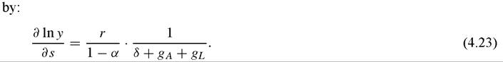
Withthe values we used above (α = 1/3, δ = 0.08, gL = 0.011 and gA = 0.015), (4.23) yields a semi-elasticity of only 1.22% when evaluated at r = 8.6%. Thus large differences in investment rates would be required to generate sizable differences in labor productivity across countries. Two differences between the way the R&D investment rate operates in our model and the way the physical capital investment rate operates in the neoclassical model stand out: first, the depreciation rate of ideas in our model is zero versus δ = 0.08 for capital in the neoclassical model; second, the elasticity of output with respect to the stock of ideas can exceed 1/3 (we have it at 2/3). To see the importance of these values, note that with α = 2/3 the semi-elasticity doubles to 2.46% (still with r = 8.6%). If we use δ = 0 as well, then the semi-elasticity increases to 9.6%. In our model, the combined share of physical capital and ideas is actually 1. Without the constraint of the world technology frontier, therefore, the long run response of output would be infinite.
It is important to recall that the results shown in Table 8 and discussed above were derived for the case of θ = 0. Is it possible that a positive value of θ could improve the model’s fit with the data? As will become clear below, countries with high levels of k and high R&D investment rates tend to cluster together. Thus, assuming a positive value for θ would actually make the model less consistent with the data, since it would imply an even larger difference between A levels across rich and poor countries.
One possible reason why the model is not doing well in matching the data is that measured R&D is not the appropriate empirical counterpart of “research” in the type of models we have been examining. In particular, measured R&D only includes formal research; this is research performed in an R&D department of a corporation or other institution. This fails to capture informal research, which may be particularly important in non-OECD countries. To explore this idea, in the rest of this section we assume that both R&D intensity and the productivity index A are measured with error. We estimate “true” R&D intensities by minimizing a loss function equal to the sum of two terms that capture, respectively, the deviation of the “true” R&D intensities from the data and the deviation of the model’s implied (log of) A values from the data, with weights given by the standard deviation of the corresponding differences.[514] In principle, we could follow this procedure for each value of θ. However, at θ = 0, the partial derivative of our loss function with respect to θ is positive and large, implying that - just as argued above - the model’s fit with the data worsens as θ increases from zero. Thus, we restrict ourselves
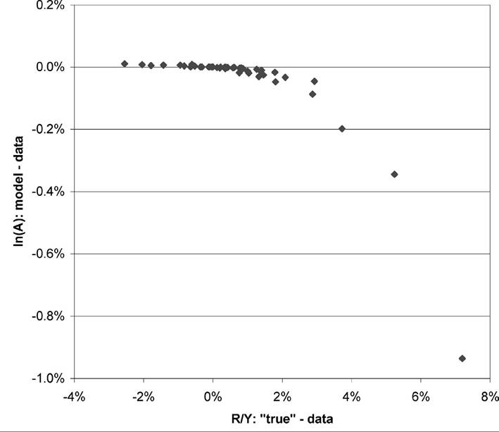
Figure 4. Deviations of the model from the data for research intensity and productivity.
to estimating R&D intensities for θ = 0 and later show what happens if, keeping the same R&D intensities estimated for θ = 0, we have positive values of θ.
It should be acknowledged that this procedure obviously implies that we can no longer evaluate the model’s consistency with the data; our interest is now to explore the implications of the model for the differences in R&D investment rates that would be necessary to explain cross-country differences in A, as well as the implied differences in R&D tax rates that would be necessary to bring about those R&D investment rates.[515]
The results of the exercise described above are shown in Figure 4 and Table 7 (columns 3 and 4). There are three points to note from these results. First, it is clear that the procedure leads to only small deviations of A from the data, whereas the deviations are more significant for R&D intensities. It would appear that R&D intensities have more significant measurement problems (or are conceptually more different than research intensity in our model) than productivity levels. Indeed, the standard deviation of residuals of sr with respect to the data is 0.12, whereas the corresponding value for the (log of) A is 0.01.[516] Second, there are some countries for which the estimated R&D intensity is much higher than the data. Italy, for example, has a measured R&D intensity of 1.1%, whereas its “true” value is 8.3%. This arises because of Italy’s high measured productivity (Italy’s A is 24% higher than the U.S. level) and low value of k (2.6 versus 3.6 in the U.S.). Something similar happens for other high-A countries, such as Hong Kong and Ireland. Finally, just as one would expect given the results above, estimated R&D intensities vary much less than the corresponding values in the data. This is the main mechanism by which the procedure allows the model to fit perfectly. It also suggests that measurement error may be behind the low R&D intensities of several poor countries and of some high A countries such as Italy, Ireland and Hong Kong.
We can now explore what happens when θ is positive, so that spillovers decline with distance. Given the estimated R&D intensities, productivity levels change with θ only because of the associated changes in the variables z, which capture the effect of distance on spillovers for each country. In principle, we can obtain the values of (z1, z2,..., z48) for any θ '≥ 0 from the solution of a system of 48 non-linear equations represented by (4.22). Equation i of this system can be expressed as:

Solving this system numerically for the parameter values we have discussed and the R&D intensities derived before, we arrive at a value of zi for each country, from which we can then obtain the country’s level of A by using Ai = aizi A from (4.18) and (4.19).
What are reasonable values to use for the parameter θ ? Using industry level data on productivity and research spending across the G-5 countries, Keller (2002) estimated a reduced form model where cumulative industry research affects own productivity and also affects productivity in the same industry in other countries through international spillovers that decline with distance.[517] Given the similarity between Keller’s system and a reduced form of our model, it seems reasonable to use Keller’s estimate of θ, namely θκ ? 0.0009 in the calibration of our model. It turns out, however, that with θ = θκ our model cannot match the data - in particular, there is no solution to the system of Equations (4.24), at least for the parameters used for the exercises above.
Table 9
Implied R&D tax rates
“True” a for
Notes: Tr is calculated as the level of Tr needed to generate the “true” research intensity. For each country, we use its own implied income tax level (tk) and its own capital intensity level k. The last column presents the equilibrium steady state relative A level (a) for the hypothetical case in which all countries have the same R&D tax as the U.S. (tr∕ = trus) but have different income tax rates and capital intensity levels.
This is because θκ is unreasonably high. One way to see this is by noting that it implies a half distance of 746 miles: this implies that spillovers from the U.S. to Japan would be only one tenth of those to Mexico, and spillovers from the U.S. to New Zealand would be only one fifth of those to Japan.
We were able to find solutions for the system with θ = θκ∕5. For comparison, we also obtained solutions for two other values of θ, namely θ = θκ∕ 10 and θ = θκ∕ 100. A group of European countries (Belgium, France, United Kingdom, Germany, Ireland, Italy, and Netherlands) always come out with the highest values of z, whereas New Zealand always comes out with the lowest value. For θ = θκ∕ 100, θ = θκ∕ 10 and θ = θκ∕5, the minimum and maximum values of z are (93%, 96%), (48%, 68%) and (24%, 50%), respectively. Clearly, for high values of θ, geography by itself can lead to large differences in productivity across countries.
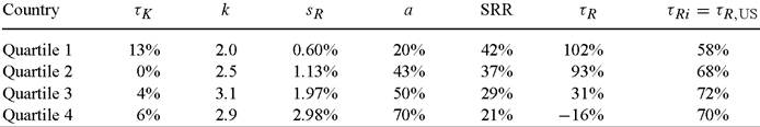
In the rest of this section, we focus on the case θ = 0, since - as explained above - the model’s fit with the data is best at this point. (Recall that the model fits perfectly because we are using the estimated research intensities and the implied A values). Table 9 presents summary statistics for the solution for the case of θ = 0. Our discussion of these results will focus on the comparison of the poorest and richest quartiles (ordered, as above, in terms of A levels) in this table.
There are several points that we want to highlight in relation to these results. First, the median income tax is 13% and 6% for the poorest and richest countries, respectively. Everything else equal, this would lead to a lower R&D investment rate in the poorest countries. Second, as expected, rich countries have a higher k than poor countries: the level of k in these two groups is 2 and 2.9, respectively. As commented in Section 4.2, higher k has a direct effect on relative A (see Equation (4.17)) and an indirect effect (it could be positive or negative) through its impact on R&D investment rates (see Equation (4.16)). A natural question arises: is it the case that once we take into account the effect of k on TFP we can resuscitate the “neoclassical revolution” mantra that differences in physical and human capital accumulation rates account for most of cross-country income differences? More concretely, how much of the variation in A
levels across countries is due to the variation in levels of k? A simple way to answer this question is to note from Equation (4.17) that differences in relative A levels are driven by differences in the product sRk across countries. Running a regression of sR on the log of this product yields a coefficient of 0.8, which implies that when sRk increases by one percent, we should expect sR to increase by 0.8%. Clearly, most of the variance of the product sRk is accounted for by the variance of sR.
Third, the social return to R&D is higher for poor countries. This is consistent with the findings in Lederman and Maloney (2003) and also with the idea that poor countries have policies and institutions that negatively affect the quantity of research.
Fourth, the column with heading tr indicates the R&D tax rate required to produce the “true” R&D investment rates given each country’s levels of τκ. The main question we address here is whether differences in income tax rates, which affect both the rate of investment in physical capital and R&D, are sufficient to explain differences in estimated research intensities. The answer is clearly negative: the required R&D tax rate in the poorest countries is 102% compared to -16% in the richest countries. To address the same question from a different angle, the last column calculates each country’s implied relative A level if all countries had the same R&D tax as the U.S. but kept their own levels of τκ. It is clear that differences in τκ alone are too small to account for the wide dispersion in productivity levels across countries.
Finally, as emphasized above, the results in Table 9 suggest that small differences in steady-state R&D investment rates have large effects on steady state relative A levels. For example, in the calibrated model, by increasing its R&D investment rate by 1% from 0.6% India could double its steady state relative A level from 17% to 34%, clearly a very large effect. India’s social rate of return to research, however, is a moderate 30%. The apparent contradiction arises because the large effect of the increase in the R&D intensity on the relative A level is a steady-state comparative-statics result, and hence does not take into account the transition, which is a crucial component in the calculation of the social rate of return to R&D. As a result, in spite of the large effect of differences in R&D investment rates on relative A levels in steady state, the required implicit taxes on R&D are not huge.
4.5. The benefits of engagement
One of the benefits of the model we have constructed is that it allows us to perform an interesting exercise. We can ask: how much do countries benefit from spillovers from the rest of the world?[518]
First, note that a country’s equilibrium ai is not affected by being isolated or engaged. Thus, the whole benefit of engagement is going to captured by the way engagement affects the term zi. Now, if a country is isolated, or disengaged, its equilibrium z would be characterized by the solution to the system (4.24) when θ → ∞. It is easy to check
27
Table 10
Benefits of engagement for selected countries
| Country | Share of world’s L | Scale effect | S.V. effect | Total effect |
| U.S. | 7.1% | 37 | 0.12 | 5 |
| UK | 1.5% | 297 | 0.21 | 64 |
| Belgium | 0.2% | 4,093 | 0.12 | 480 |
| Brazil | 3.1% | 114 | 0.97 | 110 |
| India | 1.3% | 9 | 23.0 | 217 |
| China | 38.7% | 4 | 70.6 | 258 |
| Senegal | 0.2% | 4,451 | 42.0 | 187,035 |
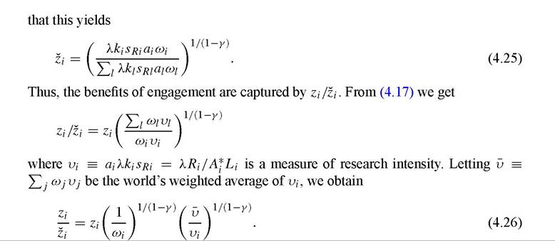
The first term on the RHS of this equation, Zi, captures the fact that even when fully engaged, a country’s technology frontier is inferior to the world’s frictionless frontier if θ > 0, in which case Zi < 1 for all i. The second term is the pure scale effect that arises in this model. The third term, which we call the “Silicon Valley” effect, captures the fact that richer countries benefit less from being part of the world than poor countries do because of their higher effective research intensity.
Table 10 presents results based on these values and assuming θ = 0, which implies Zi = 1 for all i. The results suggest huge benefits of engagement. At the extreme, Senegal’s productivity is 187 thousand times higher than it would be if it was isolated! Of course, if θ > 0 then Zi < 1 and the overall effect would be small. Still, it is our conjecture that any reasonable value of θ would still imply enormous benefits of engagement. Of course, in a more general model, it is reasonable to think that productivity could not fall below a certain level because of Malthusian forces. Specifically, suppose there is a fixed factor such as land. Then, for sufficiently low A, population would decline until income per capita was equal to the subsistence level. Instead of very low levels of A, disengagement would mean very low population sizes. Put differently, an important part of the benefits of engagement may be realized through larger population rather than higher productivity. The implications are clear: if it were not for the benefits of sharing knowledge internationally, countries would have much lower productivity levels and populations than they now do.
4.6. Discussionofmainresults
We finish this section with a discussion of the main results we want to emphasize.
First, the usual separation between capital and productivity - or between investment and technological change - is not always valid. For a given R&D investment rate, higher investment rates in physical and human capital lead naturally to higher TFP productivity levels. Thus, one should not jump from cross-country dispersion in TFP to the conclusion that differences in physical and human capital play a minority role in accounting for international income differences. When we calibrate our model, however, we find that differences in R&D investment rates account for most of the cross country variation in productivity.
Second, international variation in R&D investment appears more than large enough to generate the international variation in productivity. But it seems likely that measured R&D does not capture all of the investment associated with adoption of foreign technology. Indeed, we find that countries such as Indonesia, Peru and Senegal have R&D investment rates that are much too low to be consistent with their productivity levels. It is likely that their true research intensities are much higher than the measured ones. We hope to see more research in understanding how to capture and measure “research”.
Third, differences in (implicit) capital income tax rates are not large enough to account for the observed differences in R&D investment rates and productivity levels. The calibrated model suggests that sizable differences in R&D taxes are needed. These R&D taxes are clearly not formal or explicit taxes, but the result of policies and institutions that make research more costly or reduce its associated returns. Exploring the nature and source of these differences in implicit R&D taxes across countries is an important topic for future research.
Finally and most importantly, the calibrated model indicates that countries benefit enormously from international knowledge spillovers. We think any reasonable value of θ (which governs the rate at which spillovers decline with distance) would yield results similar to those we presented above.
5.