Cross-country evidence

In this section we document a number of facts about country growth experiences over the last fifty years. We show that country growth rates appear to depend critically on the growth and income levels of other countries, rather than solely on domestic invest­ment rates in physical and human capital.

• The growth slowdown that began in the mid-1970s was a world-wide phenomenon. It hit both rich countries and poor countries, and economies on every continent.

• Richer OECD countries grew much more slowly from 1950 to around 1980, de­spite the fact that richer OECD economies invested at higher rates in physical and human capital.

• Differences in country investment rates are far more persistent than differences in country growth rates.

• Countries with high investment rates tend to have high levels of income more than they tend to have high growth rates.

3.1. The world-wide growth slowdown

As has been widely documented for rich countries, the growth rate of productivity slowed beginning in the early 1970s.^[501] Less widely known is that the slowdown has

Table 2

Output growth declined sharply worldwide

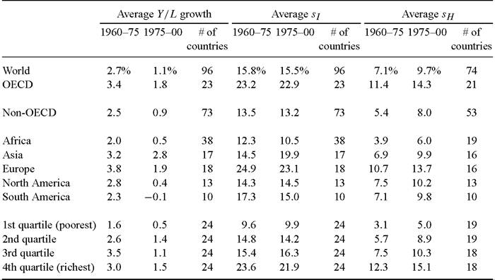
Notes: Y/L is GDP per worker. sj is the physical capital investment rate, and s∏ years of schooling attainment (for the 25+ population) divided by 60 years (working life). Data sources: Barro and Lee (2000) and Heston, Summers and Aten (2002).

been a world-wide phenomenon, rather than just an OECD-specific event.^[502] We docu­ment this in Table 2. Across 96 countries, the growth rate in PPP GDP per worker fell from 2.7% per year over 1960-1975 to 1.1% per year over 1975-2000.

Why does a world-wide growth slowdown suggest international externalities? Couldn’t it simply reflect declining investment rates world-wide, as suggested by the AK model in the previous section? Table 2 also shows what average investment rates in physical and human capital did before and after the mid-1970s. The investment rates in physical capital come from Penn World Table 6.1. As a proxy for the fraction of time devoted to accumulating more human capital, we used years of schooling attainment relative to a 60-year working life. We used data on schooling attainment for the 25 and older population from Barro and Lee (2000). This human capital investment rate, which averages around 7% across countries, reflects the fraction of ages 5 to 65 devoted to schooling as opposed to working. We prefer the attainment of the workforce as opposed to the enrollment rates of the school-age population. The latter should take a long time to affect the workforce and therefore the growth rate.

According to Table 2, the average investment rate in physical capital across all coun­tries was virtually unchanged (15.8% before vs. 15.5% after the slowdown), and the investment rate in human capital actually rose strongly (going from 7.1% to 9.7%).

The breadth of the growth slowdown suggests something linking country growth rates, and ostensibly something other than investment rates.^[504] This is contrary to the predictions of AK models, in which the growth rate of a country depends on domes­tic investment rates. The world-wide nature of the slowdown suggests that endogenous growth models, more generally, should not be applied to individual countries but rather to a collection of interdependent countries. Knowledge diffusion through trade, migra­tion, and foreign direct investment are likely sources of interdependence.

Three other examples of interdependence are offered by Parente and Prescott (2005). First, growth rates picked up in the 20th century relative to the 19th century for many countries. Second, the time it takes a country to go from $2000 to $4000 in per capita income has fallen over the 20th century, suggesting the potential to grow rapidly by adopting technology in use elsewhere. Third and related, they stress that “growth mira­cles” always occur in countries with incomes well beneath the richest countries, again consistent with adoption of technology from abroad.

Knowledge diffusion, broadly construed, could include imitation of successful in­stitutions and policies in other countries. Kremer, Onatski and Stock (2001) argue that such imitation might explain the empirical transition matrix of the world income distrib­ution. If improving institutions leads only to static gains in efficiency, however, then the barriers to imitation have to be large to explain why the best institutions are not in place everywhere. As we will illustrate in Section 4 below, the required barriers to technology adoption are modest precisely because the benefits accumulate with investments.

3.2. Beta convergence in the OECD

As documented by Baumol (1986) and many others, incomes have generally been converging in the OECD.

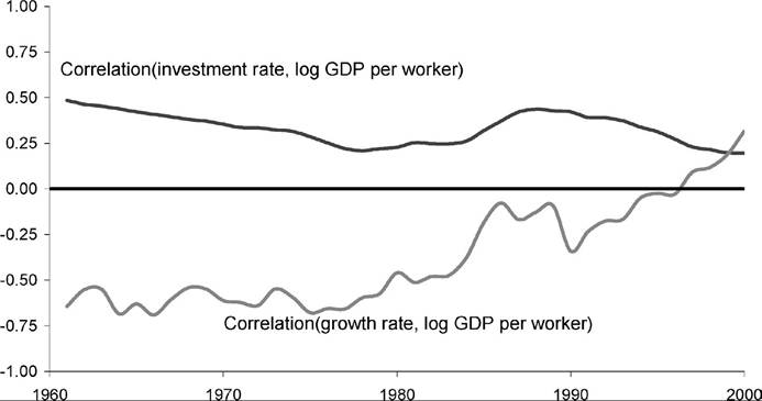
Figure 1. OECD incomes correlate negatively with growth rates, positively with investment rates. Source: Penn World Table 6.1 data on 23 OECD Countries.

vergence to describe such episodes of declining cross-sectional standard deviations in log incomes. We focus on a related concept that Barro and Sala-i-Martin labeled beta convergence, namely a negative correlation between a country’s initial income level and its subsequent growth rate. We look at beta convergence year by year in Figure 1. The data on PPP income per worker comes from Penn World Table 6.1 [Heston, Summers and Aten (2002)], and covers 23 OECD countries over 1960-2000. The figure shows the correlation between current income and growth hovering between -0.50 and -0.75 from 1960 through the early 1980s. The correlation was still negative from the mid- 1980s through the mid-1990s, but less so, and turned positive in the latter 1990s.

DeLong (1988) pointed out that a country’s OECD membership is endogenous to its level of income, so that members at time t will tend to converge toward each other’s incomes leading up to time t. Our focus, however, is not on convergence per se. Our point is instead about how investment rates correlate with income during the period of convergence. Figure 1 also shows the physical capital investment rate, and it is posi­tively correlated with a country’s income throughout the sample. Figure 2 shows that schooling attainment is also positively correlated with income throughout the sample.

How do these investment correlations square with AK-type models with no external­ities? Expression (2.15) shows that a country’s growth rate should be increasing in its investment rates. For beta convergence to occur in this model, a country’s investment rates must be negatively correlated with a country’s level of income. But Figures 1 and 2 show the opposite is true: in every year, richer OECD countries had higher investment rates in human and physical capital than poorer OECD countries did.

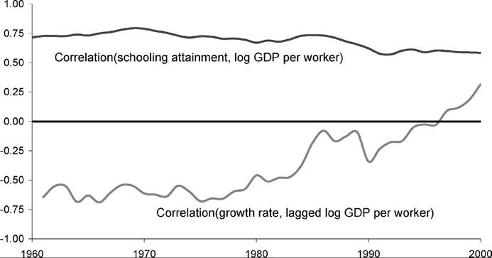
Figure 2. OECD incomes correlate negatively with growth rates, positively with investment schooling.

Source: Penn World Table 6.1 and Barro and Lee (2000) data for21 OECD Countries.

differences in efficiency parameters A and B across countries. But rescuing AK models would require that richer countries have lower efficiency parameters. We would guess that rich countries tend to have better rather than worse institutions [e.g., Hall and Jones (1999)].

3.3. Low persistence of growth rate differences

Easterly et al. (1993) documented that country growth rate differences do not persist much from decade to decade. They estimated correlations of around 0.1 to 0.3 across decades. In contrast, they found that country characteristics such as education levels and investment rates exhibit cross-decade correlations in the 0.6 to 0.9 range. Just as we do, they suggest country characteristics may determine relative income levels and world-wide technological changes long-run growth. Easterly and Levine (2001) simi­larly provide evidence that “growth is not persistent, but factor accumulation is”.

In Table 3 we present similar findings. We compare average growth rates from 1980­2000 vs. 1960-1980, and from decade to decade within 1960-2000. We find growth rates much less persistent than investment rates for the world as a whole, and for the OECD and non-OECD separately. Again, these facts seem hard to reconcile with the AK model in which a country’s domestic investment rates determine its growth rate.

Figure 3 illustrates a related pattern: deciles of countries (based on 1960 income per worker) grew at similar average rates from 1960 to 2000. Each decile consists of the unweighted average of income per worker in 9 or 10 countries.

Table 3

Investment rates are more persistent than growth rates

1980-2000 vs. 1960-1980 Decadetodecade

Notes: World = 74 countries with available data; OECD = 22 countries; and non-OECD = 52 countries. Decades consisted of the 1960s, 1970s, 1980s, and 1990s. All variables are averages over the indicated peri­ods. Each entry is from a single regression. Bold entries indicate p-values of 1% or less. Data Sources: Barro and Lee (2000) and Penn World Table 6.1 [Heston, Summers and Aten (2002)].

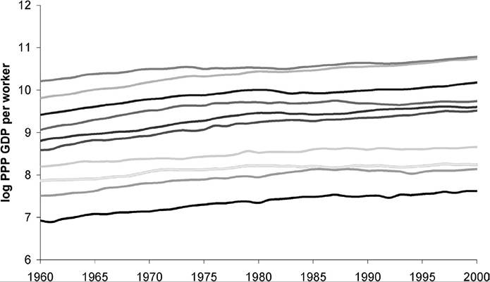
Figure 3. The evolution of income for 1960 deciles. Source: Penn World Table 6.1.

long-run growth rates, even comparing the richest and poorest countries. This sample contains 96 countries, and therefore many of the poorest countries mired in zero or negative growth.

Pritchett (1997), on the other hand, offers compelling evidence that incomes diverged massively from 1800 to 1960. Doesn’t this divergence favor models, such as AK with-

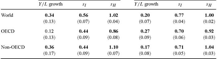
Table 4

Investment rates correlate more with levels than with growth rates

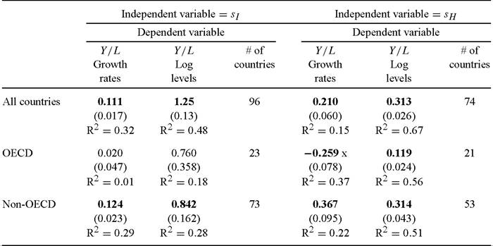
Notes: Variables are averages over 1960-2000. Each entry is from a single regression. Bold entries indicate ^-values of 1% or less. Data sources: Barro and Lee (2000) and Penn World Table 6.1 [Heston, Summers and Aten (2002)].

out international externalities, in which country growth rates are not intertwined? Not necessarily. As argued by Parente and Prescott (2005), the opening up of large in­come differences coincided with the onset of modern economic growth. The divergence could reflect the interaction of country-specific barriers to technology adoption with the emergence of modern technology-driven growth. More generally, any given divergence episode could reflect widening barriers to importing technology rather than simply dif­ferences in conventional investment rates.

3.4. Investmentratesandgrowthvs. levels

The AK model we sketched in the previous section predicts that a country’s growth rate will be strongly related to its investment rates in physical and human capital. In Table 4 we investigate this empirically in cross-sections of countries over 1960-2000. Infour of the six cases, the average investment rate is positively and significantly related to the average growth rate. For the OECD, the physical capital investment rate is not significantly related to country growth, and the human capital investment rate is actually negatively and significantly related to country growth. But for the non-OECD and all­country samples, the signs and significance are as predicted. This evidence constitutes the empirical bulwark for AK models.

In the four cases where the signs are as predicted, are the magnitudes roughly as an AK model would predict? First consider the literal AK model. According to (2.16) in the previous section, the coefficient on s_j should be A. What might be a reasonable value for A ? In order to match the average growth rate in GDP per worker (1.8%), given an average investment rate in physical capital (17%) and a customary depreciation rate (8%), the value of A would need to be

This level of A is more than four times larger than the two significant positive coef­ficients on s_j in the first column of Table 4, which are around 0.12. The estimated coefficients are small in magnitude compared to what an AK model would predict. This discrepancy could reflect classical measurement error in investment rates, but such mea­surement error would need to account for more than 80% of the variance of investment rates across countries. Plus one would expect positive endogeneity bias in estimating the average level of A, due to variation in A across countries that is positively correlated with variation in s₁.

We next consider the literal BH model. According to (2.17), the coefficient on s_H should be B.To produce the average growth rate in GDP per worker given the average investment rate in human capital (8.8%) and a modest depreciation rate (2%), B would need to be

The third column of estimates in Table 4 contain coefficients on s_H. Of the two positive coefficients, one is half the predicted level (0.21) whereas the other is not far from the predicted level (0.37).

Finally, consider the hybrid model in (2.15). We assume γ = 0.9 so that human capital accumulation is intensive in human capital, but does use some physical capital. For producing current output we assume the standard physical capital share of α = 1/3. We set the depreciation rates as previously mentioned. We set s_κ, the share of physical capital devoted to human capital accumulation, based on (2.13). As (2.15) illustrates, we cannot independently identify A and B, only their product. We set A^1-γ B^1-α = 0.60, so that the average predicted growth rate from (2.15) and observed s_H and s_j investment rates matches the average growth rate in GDP per worker of 1.8%. We then regress actual growth rates on predicted growth rates for a cross-section of 73 countries with available data. The coefficient estimated is 0.26 (standard error 0.08, R² of 0.13), far below the theoretical value of 1. Again, the empirical estimate might be low because of measurement error in predicted growth, but it would need to be large.

To recap, only 1 of the 7 coefficients of growth on investment rates considered is in the ballpark of an AK model’s prediction. In contrast, we obtain uniformly positive and significant coefficients when we regress (log) levels of country income on country investment rates. In 5 of the 6 cases, the R² is notably higher with levels than with growth rates. Investment rates appear far better at explaining relative income levels than relative growth rates. The driver of growth rates would appear to be something other than simply domestic investment rates.

The preceding discussion focused on the steady-state predictions of AK models. It is possible that AK models fare better empirically when transition dynamics are taken into account. But it is worth noting that Klenow and Rodriguez-Clare (1997), Hall and Jones (1999), Bils and Klenow (2000), Easterly (2001a), Easterly and Levine (2001), and Hendricks (2002) all find that no more than half of the variation in growth rates or income levels can be attributed directly to human and physical capital. Pritchett (2005), who considers many different parameterizations of the human capital accumulation technology, likewise finds that human capital does not account for much cross-country variation in growth rates.

3.5. R&D and TFP

We now turn away from AK models to a model with diminishing returns to physical and human capital, but with R&D as another form of investment. Such a model might be able to explain country growth rates with no reference to cross-country externalities. For example, perhaps a variant of the Romer (1990) model could be applied country by country, with no international knowledge flows. R&D investment would have to behave in a way that leads to a worldwide growth slowdown, beta convergence in the OECD, and low persistence of growth rate differences. And, more directly, R&D investment would have to explain country growth rates. Research effort, like human capital, is diffi­cult to measure. But Lederman and Saenz (2003) have compiled data on R&D spending for many countries. We now ask the same questions of their R&D investment rates that we asked of investment rates in physical and human capital: how correlated are R&D investment rates with country growth rates and country income levels?

The first column in Table 5 says that countries with high R&D spending relative to GDP do not grow systematically faster.^[505] Countries with high R&D shares do, however, tend to have high relative incomes. But the correlation with income is not significant outside the OECD. One possibility is that these regressions do not adequately control for the contributions of physical and capital. We therefore move to construct Total Factor Productivity (TFP) growth rates and levels. We subtract estimates of human and physical capital per worker from GDP per worker:

where Y is real GDP, L is employment, K is the real stock of physical capital, and H is the real stock of human capital. We suppress time and country subscripts in (3.3) for readability. We would prefer to let α vary across countries and across time based on factor shares, but such data is not readily available for most countries in the sample. We instead set α = 1 /3 for all countries and time periods. Gollin (2002) finds that capital’s

Table 5

R&D intensity also correlates more with levels than growth rates

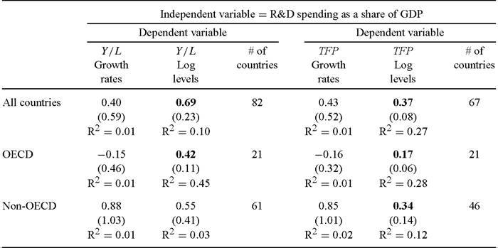
Notes: Variables are country averages over years in 1960-2000 with data relative to time effects. Y/L is GDP per worker. TFP nets out contributions from human and physical capital, as described in the text. Each entry is from a single regression. Bold entries indicate p-values of 2% or less. Data sources: Barro and Lee (2000), Penn World Table 6.1 [Heston, Summers and Aten (2002)], and Lederman and Saenz (2003).

share varies from 0.20 to 0.35 across a sample of countries, but does not correlate with country income levels or growth rates. We use Penn World Table 6.1 data assembled by Heston, Summers and Aten (2002) for PPP GDP, employment, and PPP investment in physical capital. We assume an 8% geometric depreciation rate and the usual accu­mulation equation to cumulate investment into physical capital stocks. We approximate initial capital stocks using the procedure in Klenow and Rodriguez-Clare (1997, p. 78). We let human capital per worker be a simple Mincerian function of schooling:

Here h represents human capital per worker, and s denotes years of schooling attain­ment. We use Barro and Lee (2000) data on the schooling attainment of the 25 and older population. This data is available every five years from 1960 to 2000, with the last year an extrapolation based on enrollment rates and the slow-moving stock of workers. A more complete Mincerian formulation would include years of experience in addi­tion to schooling and would sum the human capital stocks of workers with different education and experience levels. In Klenow and Rodriguez-Clare (1997) we found that taking experience and heterogeneity into account had little effect on aggregate levels and growth rates, so we do not pursue it here. We use (3.4) with the Mincerian re­turn φ = 0.085, based on the returns estimated for many countries and described by Psacharopoulos and Patrinos (2002).

The latter columns in Table 5 present regressions of TFP growth rates and levels on R&D investment rates. The sample of countries is smaller given data limitations (67 countries rather than 82). Just like growth in GDP per worker, growth in TFP is not significantly related to R&D investment rates. But TFP levels, like levels of GDP per worker, are positively and significantly related to R&D investment rates. From this we conclude that even R&D investment rates affect relative income levels, not long- run growth rates. The persistence of R&D investment rate differences across countries, combined with the lack of persistent growth rate differences, supports this interpreta­tion. We are led to consider models in which country growth rates are tethered together.

Before considering a model with international knowledge externalities, we pause to consider a model with “externalities” operating through the terms of trade. We have in mind Acemoglu and Ventura’s (2002) model of the world income distribution. In their model, each country operates an AK technology, but uses it to produce distinct national varieties. Countries with high AK levels due to high investment rates plentifully supply their varieties, driving down their prices on the world market. This results in a pAK model with a stationary distribution of income even in the face of permanent differences in country investment rates (and A levels, for that matter). Prices tether incomes together in the world distribution, not the flow of ideas. This is a clever and coherent model, but we question its empirical relevance. Hummels and Klenow (2005) find that richer countries tend to export a given product at higher rather than lower prices. They do estimate modestly lower quality-adjusted prices for richer countries, but nowhere near the extent needed to offset AK forces and generate “only” a factor of 30 difference in incomes.

To summarize this section, AK models tightly connect investment rates and growth rates. Such a tight connection does not hold empirically. This is the case for the world growth slowdown, for OECD convergence, for growth persistence, and for country vari­ation in growth vs. income levels. A version of the AK model with endogenous terms of trade might be able to circumvent these empirical hazards but faces empirical troubles of its own. We therefore turn to models with international knowledge externalities that drive long-run growth.

3.