3. Cross-country growth regressions: from theory to empirics

The stylized facts of economic growth have led to two major themes in the development of formal econometric analyses of growth. The first theme revolves around the ques­tion of convergence: are contemporary differences in aggregate economies transient over sufficiently long time horizons? The second theme concerns the identification of growth determinants: which factors seem to explain observed differences in growth? These questions are closely related in that each requires the specification of a statistical model of cross-country growth differences from which the effects on growth of various factors, including initial conditions, may be identified.

Section 3.1 provides a general theoretical framework for understanding growth dy­namics. The framework is explicitly neoclassical and represents the basis for most empirical growth work; even those studies that have attempted to produce evidence in favor of endogenous or other alternative growth theories have generally used the neo­classical model as a baseline from which to explore deviations. Section 3.2 examines the relationship between this theoretical model of growth dynamics and the specifica­tion of a growth regression. This transition from theory to econometrics produces the canonical cross-country growth regression.

3.1. Growth dynamics: basic ideas

For economy i at time t, let Y_i,_t denote output, L_i,_t the labor force (assumed to obey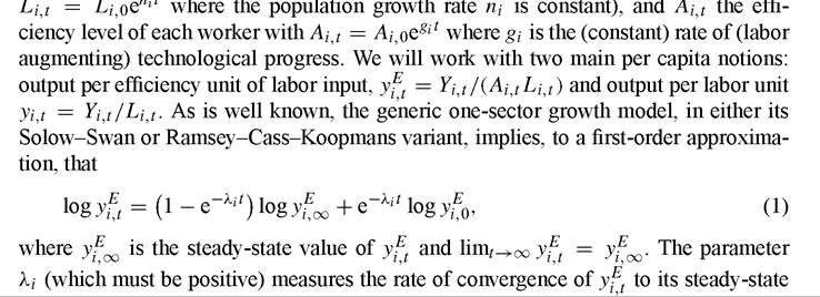

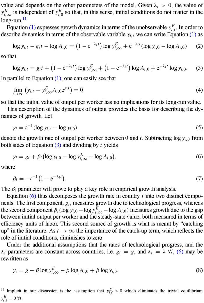
The important empirical implication of Equation (8) is that, in a cross-section of coun­tries, we should observe a negative relationship between average rates of growth and initial levels of output over any time period - countries that start out below their bal­anced growth path must grow relatively quickly if they are to catch up with other countries that have the same levels of steady-state output per effective worker and initial efficiency.

3.2. Cross-country growth regressions

^[1] We provide formal definitions of convergence in Section 4.1.

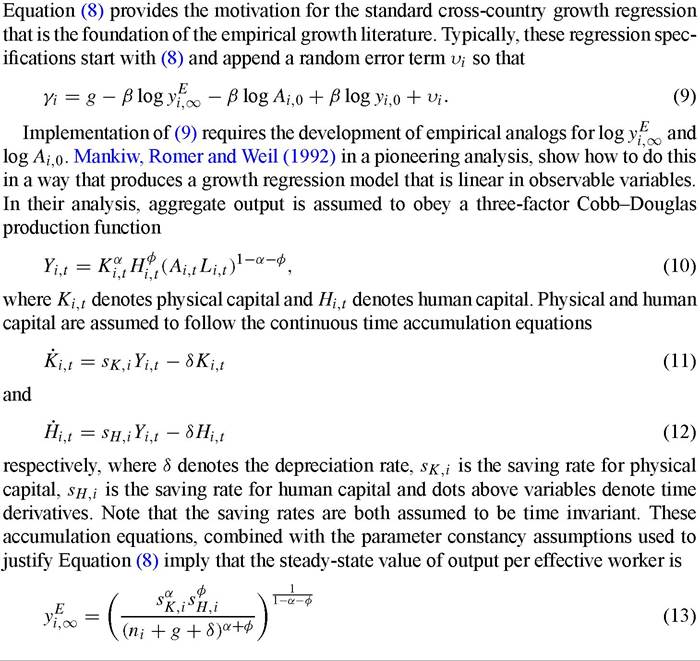
Mankiw, Romer and Weil assume that A_i,₀ is unobservable and that g + δ is known. These assumptions mean that (14) is linear in the logs of various observable variables and therefore amenable to standard regression analysis.

Mankiw, Romer and Weil argue that A_i,₀ should be interpreted as reflecting not just technology, which they assume to be constant across countries, but country-specific in­fluences on growth such as resource endowments, climate and institutions. They assume these differences vary randomly in the sense that

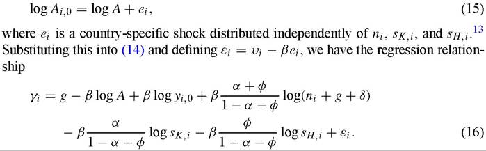
Using data from a group of 98 countries over the period 1960 to 1985, Mankiw, Romer and Weil produce regression estimates of β = -0.299, a = 0.48 and φ = 0.23.^{13 14},¹⁵ Mankiw, Romer and Weil are unable to reject the overidentifying restrictions present in (16). While this result is echoed in studies such as Knight, Loayza and Villanueva (1993), other authors, Caselli, Esquivel and Lefort (1996), for example, are able to reject the restrictions.

Many cross-country regression studies have attempted to extend Mankiw, Romer and Weil by adding additional control variables Z_i to the regression suggested by (16). Rel­ative to Mankiw, Romer and Weil, such studies may be understood as allowing for predictable heterogeneneity in the steady-state growth term gi and initial technology term A_i,₀ that are assumed constant across i in (16). Formally, the g_i — β log A_i,₀ terms

in (6) are replaced with g - β log A + πZ_i - βe_i rather than with g - β log A - βe_i which produced (16). (As far as we know, empirical work universally ignores the fact that log(n_i + g + 5) should also be replaced with log(n_i + g_i + 5).) This produces the cross country growth regression

c√ -U /7)

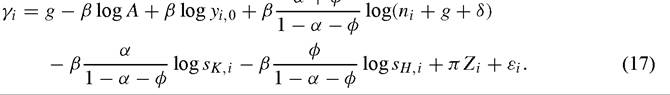
The regression described by (17) does not identify whether the controls Zi are corre­lated with steady-state growth gi or the initial technology term Ai 0. For this reason, a believer in a common steady-state growth rate will not be dissuaded by the finding that particular choices of Z_i help predict growth beyond the Solow regressors. Nevertheless, it seems plausible that the controls Z_i may sometimes function as proxies for predicting differences in efficiency growth g_i rather than in the initial technology A_{i 0}. As argued in Temple (1999), even if all countries have the same total factor productivity (TFP) growth in the long run, over a twenty- or thirty-year sample the assumption of equal TFP growth is highly implausible, so the variables in Zi can explain these differences. That being said, the attribution of the predictive content of Z_i to initial technology ver­sus steady state growth will entirely depend on a researcher’s prior beliefs.

The canonical cross-country growth regression may be understood as a version of (17) when the cross-coefficient restrictions embedded in (17) are ignored (which is usually the case in empirical work). A generic representation of the regression is

where X_i contains a constant, log(n_i∙ + g + 5), logs_κ,_i and logs_H,i. The variables spanned by log y_i, î and X_i thus represent those growth determinants that are suggested by the Solow growth model whereas Z_i represents those growth determinants that lie outside Solow’s original theory.¹⁶ The distinction between the Solow variables and Z_i is important in understanding the empirical literature. While the Solow variables usually appear in different empirical studies, reflecting the treatment of the Solow model as a baseline for growth analysis, choices concerning which Z_i variables to include vary greatly.

Equation (18) represents the baseline for much of growth econometrics. These regres­sions are sometimes known as Barro regressions, given Barro’s extensive use of such

^[1] We distinguish log y_i 0 from the other Solow variables because of the role it plays in analysis of conver­gence; see Section 4 for detailed discussion.

regressions to study alternative growth determinants starting with Barro (1991). This regression model has been the workhorse of empirical growth research.¹⁷ In modern empirical analyses, the equation has been generalized in a number of dimensions.

3.3. Interpreting errors in growth regressions

Our development of the relationship between cross-country growth regressions and neo­classical growth theories illustrates the standard practice of adding regression errors in an ad hoc fashion. Put differently, researchers usually derive a deterministic growth relationship and append an error in order to capture whatever aspects of the growth process are omitted from the model that has been developed. One problem with this practice is that some types of errors have important implications for the asymptotics of estimators. Binder and Pesaran (1999) conduct an exhaustive study of this question, one important conclusion of which is that if one generalizes the assumption of a constant rate of technical change so that technical change follows a random walk, this induces nonstationarity in many levels series, raising attendant unit root questions.

Beyond issues of asymptotics, the ad hoc treatment of regression errors leaves unan­swered the question of what sorts of implicit substantive economic assumptions are made by a researcher who does this. Brock and Durlauf (2001a) address this issue using the concept of exchangeability. Basically, their argument is that in a regression such as (18), a researcher typically thinks of the errors ε_i as interchangeable across observa­tions: different patterns of realized errors are equally likely to occur if the realizations are permuted across countries. In other words, the information available to a researcher about the countries is not informative about the error terms.

Exchangeability is a mathematical formalization of this idea and is defined as fol­lows. For each observation i, there exists an associated information set F_i available to the researcher.

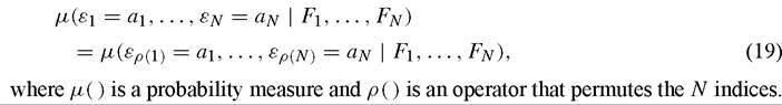
¹⁷ Such regressions appear to have been employed earlier by Grier and Tullock (1989) and Kormendi and Meguire (1985). The reason these latter two studies seem to have received less attention than warranted by their originality is, we suspect, due to their appearance before endogenous growth theory emerged as a primary area of macroeconomic research, in turn placing great interest on the empirical evaluation of growth theories. To be clear, Barro’s development is original to him and his linking of cross-country growth regressions to alternative growth theories was unique.

Many criticisms of growth regressions amount to arguments that exchangeability has been violated. For example, omitted regressors induce exchangeability violations as these regressors are elements of F. Parameter heterogeneity also leads to nonex­changeability. For these cases, the failure of nonexchangeability calls into question the interpretation of the regression. This is not always the case; heteroskedasticity in errors violates exchangeability but does not induce interpretation problems for coefficients.

Brock and Durlauf argue that exchangeability produces a link between substantive social science knowledge and error structure, i.e. this knowledge may be used to eval­uate the plausibility of exchangeability. They suggest that a good empirical practice would be for researchers to question whether the errors in a model are exchangeable, and if not, determine whether the violation invalidates the purposes for which the re­gression is being used. This cannot be done in an algorithmic fashion, but as is the case with empirical work quite generally, requires judgments by the analyst. See Draper et al. (1993) for further discussion of the role of exchangeability in empirical work.

3.