The convergence hypothesis

Much of the empirical growth literature has focused on the convergence hypothesis. Although questions of convergence predate them, recent widespread interest in the convergence hypothesis originates from Abramovitz (1986) and Baumol (1986).

In this section, we explore the convergence hypothesis. In Section 4.1 we consider the specification of notions of convergence as related to the relationship between initial conditions and long-run outcomes. Section 4.2 explores the main technique that has been employed in studying long-run dependence, β-convergence. Section 4.3 considers alternative notions of convergence that focus less on the persistence of initial conditions and instead on whether the cross-section dispersion of incomes is decreasing across time. This section explores σ-convergence, and more general notions as well as recent methods that fall under the heading of distributional dynamics. It also considers how distributional notions of convergence may be related to definitions found in Section 4.1. Section 4.4 develops time series approaches to convergence. Section 4.5 moves beyond the question of whether convergence is present to consider analyses that have attempted to identify the sources of convergence when it appears to be present.

3.1. Convergence and initial conditions

The effect of initial conditions on long-run outcomes arguably represents the primary empirical question that has been explored by growth economists. The claim that the ef­fects of initial conditions eventually disappear is the heuristic basis for what is known as the convergence hypothesis.

We first consider how to formalize the idea that initial conditions matter. While the discussion focuses on log y_ij, the log level of per capita output in country i at time t; these definitions can in principle be applied to other variables such as real wages, life expectancy, etc. Our use of log y_i,_t rather than y_i,_t reflects the general interest in the growth literature in relative versus absolute inequality, i.e. one is usually more inter­ested in whether the ratio of income between two countries exhibits persistence than an absolute difference, particularly since sustained economic growth will imply that a constant levels difference is of asymptotically negligible size when relative income is considered.

We associate with log y_i,_t initial conditions, ρ_i,0. These initial conditions do not mat­ter in the long-run if

where μ(∙) is a probability measure. To see how this definition connects with empirical growth work, note that empirical studies of convergence are often focused on whether long-run per capita output depends on initial stocks of human and physical capital.

Economic interest in convergence stems from the question of whether certain initial conditions lead to persistent differences in per capita output between countries (or other economic units). One can thus use (20) to define convergence between two economies. Let Il Il denote a metric for computing the distance between probability measures.^[323] Then countries i and j exhibit convergence if

Growth economists are generally interested in average income levels; Equation (21) implies that countries i and j exhibit convergence in average income levels in the sense

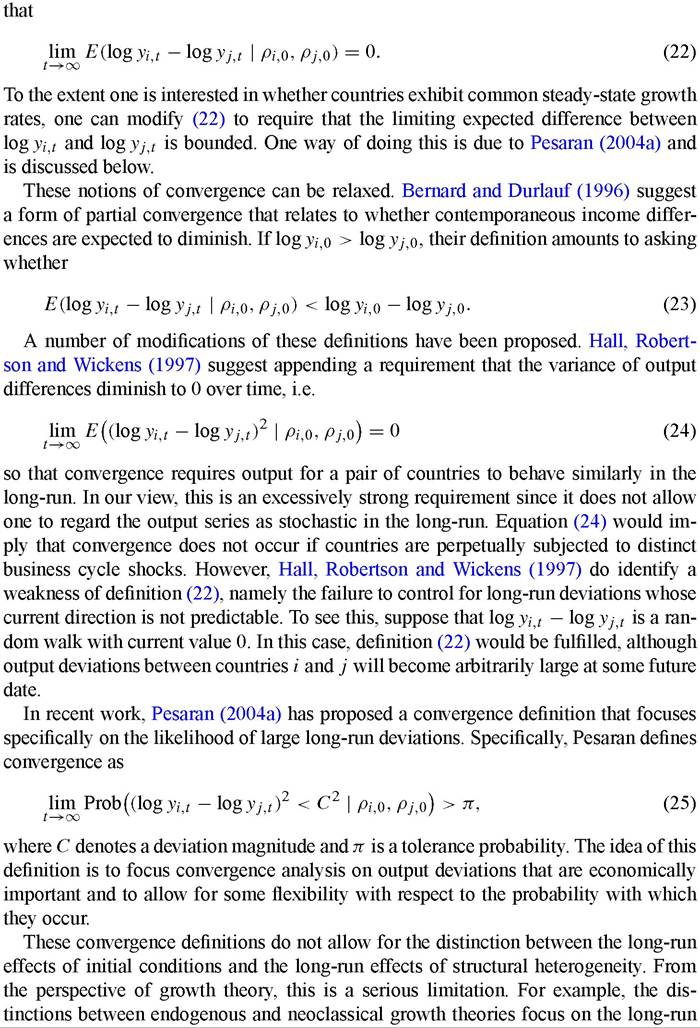
effects of cross-country differences initial human and physical capital stocks; in con­trast, cross-country differences in preferences can have long-term effects under either theory. Hence, in empirical work, it is important to be able to distinguish between initial conditions ρ_i,0 and structural characteristics θ_i,0. Steady state effects of initial condi­tions imply the existence of convergence clubs whereas steady-state effects of structural characteristics do not. In order to allow for this, one can modify (21) so that

implies that countries i and j exhibit convergence. The notions of convergence in ex­pected value (Equation (22)) may be modified in this way as well,

as can partial convergence in expected value (Equation (23)) and the other convergence concepts discussed above.

In practice, the distinction between initial conditions and structural heterogeneity generally amounts to treating stocks of initial human and physical capital as the for­mer and other variables as the latter.

The translation of these ideas into restrictions on growth regressions has led to a range of statistical definitions of convergence which we now examine. Before doing so, we emphasize that none of these statistical definitions is necessarily of intrinsic interest per se; rather each concept is useful only to the extent it elucidates economically interesting notions of convergence such as Equation (20). The failure to distinguish between convergence as an economic concept and convergence as a statistical concept has led to a good deal of confusion in the growth literature.

4.2. β-convergence

Statistical analyses of convergence have largely focused on the properties of β in re­gressions of the form (18). β -convergence, defined as β < 0 is easy to evaluate because it relies on the properties of a linear regression coefficient. It is also easy to interpret in the context of the Solow growth model, since the finding is consistent with the dy­namics of the model. The economic intuition for this is simple. If two countries have common steady-state determinants and are converging to a common balanced growth path, the country that begins with a relatively low level of initial income per capita has a lower capital-labor ratio and hence a higher marginal product of capital; a given rate of investment then translates into relatively fast growth for the poorer country. In turn, β -convergence is commonly interpreted as evidence against endogenous growth models of the type studied by Romer and Lucas, since a number of these models specifically

predict that high initial income countries will grow faster than low initial income coun­tries, once differences in saving rates and population growth rates have been accounted for.

There now exists a large body of studies of β -convergence, studies that are differ­entiated by country set, time period and choice of control variables. When controls are absent, β < 0 is known as unconditional β-convergence: conditional β-convergence is said to hold if β < 0 when controls are present. Interest in unconditional β -convergence, while not predicted by the Solow growth model except when countries have common steady-state output levels, derives from interest in the hypothesis that all countries are converging to the same growth path, which is critical in understanding the extent to which current international inequality will persist into the far future.^[325] Typically, the unconditional β -convergence hypothesis is supported when applied to data from rela­tively homogeneous groups of economic units such as the states of the US, the OECD, or the regions of Europe; in contrast there is generally no correlation between initial income and growth for data taken from more heterogeneous groups such as a broad sample of countries of the world.^[326]

Many cross-section studies employing the β -convergence approach find estimated convergence rates of about 2% per year.^[327] This result is found in data from such diverse entities as the countries of the world (after the addition of conditioning variables), the OECD countries, the US states, the Swedish counties, the Japanese prefectures, the regions of Europe, the Canadian provinces, and the Australian states, among others; it is also found in data sets that range over time periods from the 1860’s though the 1990’s^[328] Some writings go so far as to give this value a status analogous to a universal

constant in physics.^[329] In fact, there is some variation in estimated convergence rates, but the range is relatively small; estimates generally range between 1% and 3%, as noted by Barro and Sala-i-Martin (1992).^[330]

Despite the many confirmations of this result now in the literature, the claim of global conditional β-convergence remains controversial; here we review the primary problems with the β-convergence literature.

4.2.1. Robustness with respect to choice of control variables

Inmovingfromunconditionalto conditional β-convergence, complexities arise in terms of the specification of steady-state income. The reason for this is the dependence of the steady-state on Z. Theory is not always a good guide in the choice of elements of Z; differences in formulations of Equation (18) have led to a “growth regression industry” as researchers have added plausibly relevant variables to the baseline Solow specification. As a result, one can identify variants of (18) where convergence appears to occur as β3 < 0 as well as variants where divergence occurs, i.e. β3 > 0.

We discuss issues of uncertainty in the specification of growth regressions below. Here we note here that one class of efforts to address model uncertainty has led to con­firmatory evidence of conditional β -convergence. This approach assigns probabilities to alternative formulations of (18) and uses these probabilities to construct statements about β that average across the different models. Doppelhofer, Miller and Sala-i-Martin (2004) conclude the posterior probability that initial income is part of the linear growth model is 1.00 with a posterior expected value for β of -0.013; this leads to a point estimate of a convergence rate of 1.3% per annum, which is somewhat lower than the 2% touted in the literature; Fernandez, Ley and Steel (2001a) also find that the posterior probability that initial income is part of the linear growth model is 1.00, despite using a different set of potential models and different priors on model parameters.^[331] We there­fore conclude that the evidence for conditional β -convergence appears to be robust with respect to choice of controls.

4.2.2. Identification and nonlinearity: β-convergence and economic divergence

A second problem with the β-convergence literature is an absence of attention to the relationship between β -convergence and economic convergence as defined by Equa­tion (20) or variations based upon it. Put differently, in the β -convergence literature there is a general failure to develop tests of the convergence hypothesis that discrim­inate between convergent economic models and a rich enough set of non-converging alternatives.

While β < 0 is an implication of the Solow growth model and so is an implication of the baseline convergent growth model in the literature, this does not mean that β < 0 is inconsistent with economically interesting non-converging alternatives. One such ex­ample is the model of threshold externalities and growth developed by Azariadis and Drazen (1990). In this model, there is a discontinuity in the aggregate production func­tion for aggregate economies. This discontinuity means that the steady-state behavior of a given economy depends on whether its initial capital stock is above or below this threshold; specifically, this model may exhibit two distinct steady states. (Of course, there can be any number of such thresholds.) An important feature of the Azariadis- Drazen model is that data generated by economies that are described by it can exhibit statistical convergence even when multiple steady states are present.

To illustrate this, we follow an argument in Bernard and Durlauf (1996) based on a simplified growth regression. Suppose that for every country in the sample, the Solow variables X_i and additional controls Z_i are identical. Suppose as well that there is no technical change or population growth. Following the standard arguments for deriving a cross-country regression specification, the growth regression implied by the Azariadis- Drazen assumption on the aggregate production function is

where l(i) indicates the steady state with which country i is associated and y^-.) denotes output per capita in that steady state; all countries associated with the same steady state thus have the same log y*(_i) value.

The threshold externality model clearly does not exhibit economic convergence as defined above so long as there are at least two steady states. Yet the data generated by a cross-section of countries exhibiting multiple steady states may exhibit statistical convergence. To see this, notice that for this stylized case, the cross-country growth regression may be written as

Since the data under study are generated by (28), this standard regression is misspec­ified. What happens when (29) is estimated when (28) is the data generating process? Using population moments, the estimated convergence parameter β_ols will equal

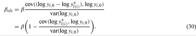
From the perspective of tests of the convergence hypothesis, the noteworthy fea­ture of (30) is that one cannot determine the sign of β_ols a priori as it depends on 1 - cov(log y*(_i), log y_i,o)∕var(log y_i,₀), which is a function of the covariance between the initial and steady-state incomes of the countries in the sample. It is easy to see that it is possible for β_ols to be negative even when the sample includes countries associated with different steady states. Roughly speaking, one would expect β_ols < 0 if low-income countries tend to initially be below their steady states whereas high-income countries tend to start above their steady states. While we do not claim this is necessarily the case empirically, the example does illustrate how statistical convergence (defined as β < 0) may be consistent with economic nonconvergence. Interestingly, it is even possible for the estimated convergence parameter β_ols to be smaller (and hence imply more rapid convergence) than the structural parameter β in (28).

Below, we review evidence of multiple steady states in the growth process. At this stage, we would note two things. First, some studies have produced evidence of multiple regimes in the sense that statistical models consistent with multiple steady states appear to better fit the cross-country data than the linear Solow model, e.g., Durlauf and John­son (1995). Second, other studies have produced evidence of parameter heterogeneity such that β appears to depend nonlinearly on initial conditions so that it is equal to 0 for some countries; Liu and Stengos (1999) find precisely this when they reject the spec­ification of constant β for all countries in favor of a specification in which β depends on initial income. These types of findings imply the compatibility of observed growth patterns with the existence of permanent income differences between economies with identical population growth and savings rates and access to identical technologies.

4.2.3. Endogeneity

A third criticism that is sometimes made of the empirical convergence literature is based on the failure to account for the endogeneity of the explanatory regressors in growth regressions. One obvious reason why endogeneity may matter concerns the consistency of the regression estimates. This concern has led some authors to propose instrumental variables approaches to estimating β. Barro and Lee (1994) analyze growth data in the periods 1965 to 1975 and 1975 to 1985 and use 5-year lagged explanatory variables as instruments. Barro and Lee find that the use of instrumental variables has little effect on coefficient estimates. Caselli, Esquivel and Lefort (1996) employ a generalized method of moments (GMM) estimator to analyze a panel variant of the standard cross-country growth regression; growth in the panel is measured in 5-year intervals for 1960-1985. Their analysis produces estimates of β on the order of 10%, which is much larger than the 2% typically found.

Endogeneity raises a second identification issue with respect to the relationship be­tween β-convergence and economic convergence: this idea appears in Cohen (1996) and Goetz and Hu (1996). Focusing on the Solow regressors, the value of β can fail to illustrate how initial conditions affect expected future income differences if the pop­ulation and saving rates are themselves functions of income. Hence, β f 0 may be compatible with at least partial economic convergence, if the physical and human cap­ital savings rates depend, for example, on the level of income. In contrast, β < 0 may be compatible with economic divergence if the physical and human capital accumula­tion rates for rich and poor are diverging across time. As such, this critique is probably best understood as a debate over what variables are the relevant initial conditions for evaluating (22) and/or (23). Cohen (1996) argues that the conventional human capital accumulation equation, in which accumulation is proportional to per capita output, is misspecified, failing to account for feedbacks from the stock of human capital to the accumulation process. This feedback means that poor countries with low initial stocks of human capital fail to accumulate human capital as quickly as richer ones. Goetz and Hu (1996) directly focus on the feedback from income to human capital accumulation.

The implications of this form of endogeneity for empirical work on convergence are mixed. Cohen (1996) concludes that a proper accounting for the dependence of human capital accumulation on initial capital stocks reconciles conditional β-convergence with unconditional β -divergence for a broad cross-section. Goetz and Hu (1996), in contrast, find that estimates of the speed of convergence are increased if one accounts for the effect of income on human capital accumulation for counties in the US South. This seems to be an area that warrants much more work.

4.2.4. Measurement error

As Abramovitz (1986), Baumol (1986), DeLong (1988), Romer (1990), and Temple (1998) point out, measurement errors will tend to bias regression tests towards results consistent with the hypothesis of β -convergence. This occurs because, by construction, γ_it is measured with positive (negative) error when log y_i,₀ is measured with negative (positive) error so there tends to be a negative correlation between the measured values of the two variables even if there is none between the true values. To see this, we ignore the issue of control variables and consider the case where growth is described by γ_i = k + β log y_i,î + ε_i where ε_i is independent across observations. Suppose that log output is measured with error so that the researcher only observes ς_i^_t = log y_i,_t + e_iyt, t = 0,T where e_it is a serially uncorrelated random variable with variance σ2 and distributed independently of log y_is and ε_i for all i and s. The regression of observed growth rates will, under these assumptions, obey the equation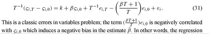

of observed growth rates on observed initial incomes will tend to produce an estimated coefficient that is consistent with the β -convergence hypothesis even if the hypothesis is not reflected in the actual behavior of growth rates across countries. In practice, as Temple (1998) explains, the direction of the bias is made ambiguous by the possibilities that the e^_t are serially dependent and that other right-hand-side (conditioning) variables are also measured with error. The actual effect of measurement error on results then becomes an empirical matter to be investigated by individual researchers.

In studying the role of the level of human capital in determining the rate of growth, Romer (1990) estimates a growth equation that has among its explanatory variables the level of per capita income at the beginning of the sample period. Consistent with the conditional β-convergence hypothesis, he finds a negative and significant coefficient on this variable when the equation is estimated by ordinary least squares. Wary of the possibility and effects of measurement error in initial income, as well as in the human capital variable - the literacy rate - Romer also estimates the equation using the number of radios per 1000 inhabitants and (the log of) per capita newsprint consumption as instruments for initial income and literacy with the result that the coefficients on both variables become insignificant “suggesting” that the OLS results are “attributable to measurement error” (p. 278).

Temple (1998) uses the measurement error diagnostics developed by Klepper and Leamer (1984) and Klepper (1988), in addition to classical method-of-moments ad­justments, to investigate the effects of measurement error on the estimated rate of convergence in Mankiw, Romer and Weil augmented Solow model. He finds that al­lowing for the possibility of small amounts of unreliability in the measurement of initial income implies a lower bound on the estimated convergence rate just above zero - too low to elevate conditional convergence to the status of a stylized fact. Barro and Sala-i-Martin (2004, pp. 472-473) use lagged values of state personal income as in­struments for initial income to check for the possible effects of measurement error in their β-convergence tests for the US states. They find little change in the estimated con­vergence rates and conclude that measurement error is not an important determinant of their results. Barro (1991) follows the same procedure for other data sets and reaches a similar conclusion about the unimportance of measurement error in his results.

Some authors have attempted to address the sources of measurement error. Dowrick and Quiggin (1997) is a notable example in this regard in their consideration of the role of price indices in affecting convergence tests. Specifically, they examine the effect of constant price estimates of GDP on β -convergence calculations and find that when the prices used to construct these measures are based on prices in advanced economies, tendencies towards convergence are understated.

4.2.5. Effects of linear approximation

There is a body of research that explores the effects of the approximations that are employed to produce the linear regression models used to evaluate β-convergence. As outlined earlier, regression tests of the β -convergence hypothesis rely on a log-linear approximation to the law of motion in a one sector neoclassical growth model. In ad­dition to the possibility that Taylor series approximations in the nonstochastic version of the model are inadequate, Binder and Pesaran (1999) show that the standard practice of adding a random term to the log-linearized solution of a nonstochastic growth model does not necessarily produce the same behavior as associated with the explicit solution of a stochastic model.

Efforts to explore the limits of the linear approximation used in empirical growth studies have generally concluded that the approximation is reasonably accurate. Romer (2001, p. 25, n. 18) claims that the approximation will be “quite reliable” in this context and Dowrick (2004) presents results showing that the approximation to the true transi­tion dynamics is quite good in a Solow model with a single capital good and an elasticity of output with respect to capital of 2/3. This is larger than the typical physical capital share but it is not an unreasonable number for the sum of the shares of physical and human capital. To test for nonlinearity, Barro (1991) adds the square of initial (1960) income to one of his regressions and finds a positive estimated coefficient implying that the rate of convergence declines as income rises and that it is positive only for incomes below $10800 - a figure that exceeds all of the 1960 income levels in his sample. How­ever, the t-ratio for the estimated coefficient on the square of initial income is just 1.4 which represents weak evidence against the adequacy of the approximation.

How should one interpret such findings? At one level, these studies conclude that the approximation used to derive the equation used in cross-section convergence studies appears to be reasonably accurate. It follows that the previously discussed nonlineari­ties in the growth process found by researchers investigating the possibility of multiple steady states do not reflect the inadequacy of the linear approximation used in most cross-section studies. Put differently, evidence of nonlinearity appears to reflect deeper factors than simple approximation error from the use of a first order Taylor series ex­pansion.

4.3. Distributional approaches to convergence

A second approach to convergence focuses on the behavior of the cross-section distribu­tion of income in levels. Unlike the ^-convergence approach, the focus of this literature has been less on the question of relative locations within the income distribution, i.e. whether one can expect currently poor countries to either equal or exceed currently af­fluent countries, but rather on the shape of the distribution as a whole. Questions of this type naturally arise in microeconomic analyses of income inequality, in which one may be concerned with whether the gap between rich and poor is diminishing, regardless of whether the relative positions of individuals are fixed over time.

4.3.1. σ -convergence

Much of the empirical literature on the cross-country income distribution has focused on the question of the evolution of the cross-section variance of log y^_t. For a set of income levels let σ_l0_{g y t} denote the variance across i of log y_ij. σ -convergence is said to hold between times t and t + T if

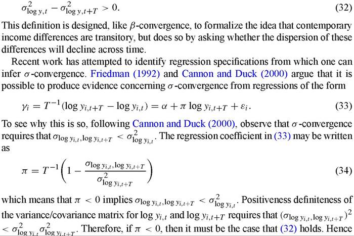
a test that accepts the null hypothesis that π < 0 by implication accepts the null hy­pothesis of σ -convergence. But even this type of test has some difficulties. As pointed out by Bliss (1999, 2000), it is difficult to interpret tests of σ -convergence since these tests presume that the data generating process is not invariant; an evolving distribution for the data makes it difficult to think about test distributions under a null. Additional issues arise when unit roots are present.

One limitation to this approach is that it is not clear how one can formulate a sensible notion of conditional σ-convergence. A particular problem in this regard is that one would not want to control for initial income in forming residuals, which would render the concept uninteresting as it could be generated by nothing more than time-dependent heteroskedasticity in the residuals. On the other hand, omitting income would render the interpretation of the projection residuals problematic since initial income is almost certain to be correlated with the variables that have been included when the residuals are formed. An economically interesting formulation of conditional σ -convergence would be a useful contribution.

4.3.2. Evolution of the world income distribution

Work on σ -convergence has helped stimulate the more general study of the evolution of the world income distribution. This work involves examining the cross-section dis­tribution of country incomes at two or more points in time in order to identify how this cross-section distribution has changed. Of particular interest in such studies is the presence or emergence of multiple modes in the distribution. Bianchi (1997) uses non­parametric methods to estimate the shape of the cross-country income distribution and to test for multiple modes in the estimated density. He finds evidence of two modes in densities estimated for 1970, 1980, and 1989. Moreover, he finds a tendency for the modes to become more pronounced and to move further apart over time. This evidence supports the ideas of a vanishing middle as the distribution becomes increasingly polar­ized into “rich” and “poor” and of a growing disparity between those two groups. While such polarization might be desirable, were it the case that middle income economies were becoming high income ones, Bianchi’s evidence suggests that much of this move­ment represents a transition from middle income to poor. Further, by “cutting” each of the estimated densities at the anti-mode between the two modes, Bianchi is able to mea­sure mobility within the distribution by counting the crossings of the cut points. These crossings represent countries moving from one basin of attraction to the other. Just 3 of the possible 238 crossings are observed.^[332] The implication is that there is very lit­tle mobility within the cross-country income distribution. The 20 or so countries in the “rich” basin of attraction in 1970 are still there in 1989 and similarly for the 100 or so countries starting in the “poor” basin.

Paap and van Dijk (1998) model the cross-country distribution of per capita income as the mixture of a Weibull and a truncated normal density. The Weibull portion captures the left-hand mode and right skewness in the data while the truncated normal portion captures the right-hand mode. This combination is selected after testing the goodness of fit of various combinations of the normal density (truncated at zero), gamma, log normal and Weibull distributions; the data set that is employed measures levels of real GDP per capita for 120 countries for the time period 1960 and 1989. They find a bimodal fitted density in each year with “poor” and “rich” components corresponding to the Weibull and truncated normal densities respectively. The computed means of these components diverge over the sample period and the weight given to the poor component in the mix­ture jumps in the mid-1970's from about 0.72 to about 0.82 implying that the mean gap between rich and poor countries grew and the poor increased in number. The attention to levels rather than log levels makes it hard to evaluate the welfare significance of this increased dispersion.

Recently, analyses of the distributions of income and growth have focused on iden­tifying differences in these distributions across time and across subsets of countries. Anderson (2003) studies changes in the world income distribution by using nonpara­metric density function estimates combined with stochastic dominance arguments to compare the distributions at different points in time.^[333] These methods allow him to con­struct measures of polarization of the income distribution; polarization is essentially characterized by shifts in probability density mass that increase disparities between relatively rich and relatively poor economies. Anderson finds that between 1970 and 1995 polarization between rich and poor countries increased throughout the time pe­riod. Maasoumi, Racine and Stengos (2003) analyze the evolution of the cross-country distributions of realized, predicted, and residual growth rates; fitted growth rates and residuals are formed from nonparametric growth regressions using the Solow variables. These authors find that the distributions of growth rates for OECD and non-OECD countries are persistently different between 1965 and 1995, with the OECD distribu­tion’s variance reducing over time whereas the non-OECD distribution appears to be becoming less concentrated. One finds the same results for fitted growth rates; in con­trast it is difficult to identify dimensions along which the distributions of OECD and non-OECD growth rate residuals differ. The major methodological difference between these papers relative to Paap and van Dijk (1998) is that these analyses do not rely on a mixture specification.

Distributional approaches suggest the utility of convergence measures that are based on the complete properties of probability measures characterizing output for different economies. Letting μ_i(x) and μj(x) denote the probability density functions for the variable of interest in economies i and j respectively, Anderson and Ge (2004) propose computing the convergence statistic CI_i j

This statistic is bounded between 0 and 1; a value of zero means that the density func­tions never assign positive probability to any common intervals or values of x whereas a value of 1 means that the densities coincide on all positive probability intervals or val­ues. Andersonand Ge (2004) refer to the case CI_i j = 1 as complete convergence. This statistic differs from the convergence measure described by Equation (21) as it evalu­ates differences between current densities and not asymptotic ones, but they are clearly closely related.

In our view, this approach will likely prove useful in a range of contexts. In particu­lar, if one is interested in comparing income distributions between two economies, the Anderson-Ge statistic is a natural metric. In growth contexts, it is less clear whether the higher moments that distinguish (22) from (35) are of major concern, at least in the context of current debates.

4.3.3. Distribution dynamics

In a series of papers, Quah (1993a, 1993b, 1996a, 1996b, 1996c, 1997) has persuasively criticized standard regression approaches to studying convergence issues for being un­able to shed light on important issues of mobility, stratification, and polarization in the world income distribution. Rather than studying the average behavior of a representative country, Quah proposes a schema, which he calls “distribution dynamics”, for studying the evolution of the entire cross-country income distribution. One way of implementing this approach is to assume that the process describing the evolution of the distribution is time-invariant and first-order Markov. Discretizing the state space then permits rep­resentation of the cross-country income distribution as a probability mass function, λ_t, with an associated transition matrix, M. Each row of M is a probability mass function describing the distribution over states of the system after one transition given that the system is currently in the state corresponding to that row. The evolution of the income distribution can then be described by λ_t = M'λ_t-1 so that λ_t+s = (M^s')'λ_t is the s- step-ahead probability mass function and λ∞ = M'λ∞ defines the long-run (ergodic) mass function (if it exists). Quah (1993b, 1996b) takes this approach and finds that the estimated M implies a bimodal (“twin-peaked”) ergodic mass function indicating a tendency towards polarization in the evolution of the world income distribution.^[334]

Updating Quah’s analysis using more recent data, Kremer, Onatski and Stock (2001) also find evidence of twin-peaks in the long-run distribution of per capita incomes. However, they find the rich (right-hand) peak to be much larger than the poor (left-hand) peak unlike Quah, who found similarly sized peaks at both ends of the distribution. Kremer, Onatski and Stock’s point estimates imply that most countries will ultimately move to the rich state although, during the transition period, which could last hundreds of years, polarization in the income distribution may worsen. They are also unable to reject the hypothesis that there is a single right-hand peak in the long-run distribution. Quah (2001) responds to these claims by arguing that the imprecision in the estimates of the ergodic distributions is such that it is not possible to reject a wide range of null hypotheses including, by construction, that of twin-peakedness. Importantly, as Quah notes his work and that of others, including Kremer, Onatski and Stock, is consistent with the view that the global poor are many in number and likely to be so for a very long time.

In addition, as Quah (1996c, 1997, 2001) and Bulli (2001) discuss, the process of discretizing the state space of a continuous variable is necessarily arbitrary and can al­ter the probabilistic properties of the data. Especially relevant here is the fact that the shape of the ergodic distribution can be altered by changing the discretization scheme. Reichlin (1999) demonstrates that the dynamic behavior inferred from the analysis of Markov transition probabilities, and the apparent long-run implications of that behav­ior, are sensitive to the discretization scheme employed; this work also shows that the estimated ergodic distribution can be sensitive to small changes in the transition proba­bilities. Bulli (2001) addresses this critique and shows how to discretize the state space in a way that preserves the probabilistic properties of the data. Applying her method to cross-country income data she finds an estimated ergodic distribution quite different from that found by arbitrary discretization as well as being an accurate approximation to the distribution computed using a continuous state space method.

An alternative formulation of distribution dynamics that avoids discretization prob­lems is proposed by Quah (1996c, 1997) and models the cross-country income distrib­ution at time t with the density function, f_t(x). If the process describing the evolution of the distribution is again assumed to be time-invariant and first-order Markov, then density at time t + τ, τ > 0, will be ft+_r(x) = ∕₀∞ g_τ(x∖z)ft(z) dz where g_τ(x∖z) is the τ-period-ahead density of x conditional on z. The function g_τ (x ∖z) is the continuous analog of the transition matrix M and, assuming it exists, the ergodic (long-run) density function, f∞ (x), implied by g_τ (x |z) is the solution to f∞ (x) = J0∞ g_τ (x ∖z)f∞ (z) dz. Using nonparametric methods, Quah (1996c, 1997) estimates various g_τ (x ∖z) and finds strong evidence of twin-peakedness in the cross-country income distribution. The esti­mated ergodic densities presented by Bulli (2001) and Johnson (2004) support Quah’s conclusions.

Azariadis and Stachurski (2003) derive the form of the g_τ(x ∖z) implied by a stochastic version of the model in Azariadis and Drazen (1990). Estimation of the model’s para­meters enables them to compute forward projections of the sequence of cross-country income distributions, and ultimately the ergodic distribution, implied by the model. Consistent with the work of Quah (1996c, 1997) they find bimodality to be a perva­sive feature of the sequence of distributions for about 100 years. Eventually, however, all countries transition to the rich mode so the ergodic distribution is unimodal as found by Kremer, Onatski and Stock (2001). As Quah (2001) notes, there is “as yet” no theory of inference for this case so reconciliation of this result with the view that the ergodic distribution is bimodal cannot be done through formal statistical tests. However, while Quah (2001) observes that such a theory is an “obvious next step”, he suggests that we may be close to the limits of what can be reasonably inferred from the cross-country income data.

Johnson (2000) offers an interpretation of g_τ(x∖z) which draws an analogy between the median of the conditional distribution and the law of motion of a non-stochastic one- variable dynamic system. The median is the function m(x) such that ∕m(^x) g_τ (z∖x) dz = 0.5 so that a country with income of m(x) at time t has an equal chance of having a higher or lower income at time t + τ. Consider a point x₀ such that m(x₀) = x₀ and suppose that, in some neighborhood of x₀, m(x) > x for x < x₀ and m(x) < x for x > x₀ implying Pr(x_t+_τ > x_t) > 0.5 for x < x₀ and Pr(x_t+_τ < x_t) > 0.5 for x > x₀ so that, in this neighborhood, countries with incomes different from x₀ tend to move toward x0. In the long run we may expect to find many countries in the vicinity of x₀ creating the tendency for a mode in the ergodic density, f∞(x), at x₀. Similarly, in a non-stochastic one-variable dynamic system with the law of motion x_t+τ = m(x_t), the condition on the phase diagram for the local stability of a steady-state at χ₀ is that the graph of m(x) intersects the 45^o line from above at x₀. In both cases, x₀ is a point of accumulation in the sense that the long-run probability of finding countries in the vicinity of x₀ will tend to be high relative to that elsewhere. Conversely, just as steady states are unstable in the non-stochastic case when m(x) crosses the 45^o line from below, analogous points in the stochastic case tend to produce antimodes in the ergodic density.

While Quah’s estimated g_τ (x |z) indicate a strong tendency towards polarization in the world income distribution, they do not reveal much about intra-distribution mobil­ity. Bimodality is arguably of less concern in a normative sense if there is movement between the two modes than it is if there is none. Quah (1996c) studies the mobility within the distribution by computing, (through stochastic simulation) the mean time for a “growth miracle” which he defines as passage from the 10th to 90th percentile of the distribution. He finds an expected time of 201 years for such a miracle to occur.

Quah’s methods have subsequently been applied to a range of contexts. Andres and Lamo (1995) apply these methods to the OECD, Lamo (2000) to the regions of Spain, Johnson (2000) to US states, Bandyopadhyay (2002) to the Indian states, and Andrade et al. (2004) to Brazilian municipalities. These methods have also been extended to broader notions of distributional dynamics. Fiaschi and Lavezzi (2004) develop an analysis of the joint distribution of income levels and growth rates; their findings are compatible with the existence of multiple equilibria in the sense that countries may become trapped in the lower part of the income distribution.

4.3.4. Relationship between distributional convergence and the persistence of initial conditions

Distributional methods have proved important in establishing stylized facts concerning the world income distribution. At the same time, there has been relatively little for­mal effort to explore the implications of findings such as twin peaks for the empirical salience of alternative growth theories. Some potential implications of distributional dynamics for evaluating theories are suggested by Quah (1996c), who finds that condi­tioning on measures of physical and human capital accumulation similar to those used by Mankiw, Romer and Weil (1992) and a dummy variable for the African continent has little effect on the dynamics of the cross-country income distribution. The polar­ization and immobility features are similar in both cases and conditioning increases the expected time for a growth miracle to 760 years.^[335] These results suggest that the hetero­geneity revealed by the distributional approaches is, at least in part, due to the existence of convergence clubs.

That being said, in general, it is relatively difficult to interpret properties of the cross­country income distribution in the context of economic convergence in the sense of (22). To see why this is so, it is useful to focus on the absence of a clear relationship between β-convergence, which measures the relative growth of rich versus poor countries and σ -convergence, which focuses explicitly on the distribution of countries. These two con­vergence notions do not have any necessary implications for one another, i.e. one may hold when the other does not. For our purposes, what is important is that σ -convergence is not an implication of β -convergence and so does not speak directly to the question of the transience of contemporary income differences. The erroneous assertion that β - convergence implies σ -convergence is known as Galton’s fallacy and was introduced into the modern economic growth context by Friedman (1992) and Quah (1993a).

To understand the fallacy, suppose that log per capita output in each of N countries obeys the AR(1) process

where 0 < ς < 1 and the random variables εy_t are i.i.d across countries and time. For this model, each country will, by definition (22), exhibit convergence as any contempo­raneous difference in output between two countries will disappear over time. Further, it is easy to see, using γ_i = T^—1(logyy_t+τ — log yty), that the regression of growth on a constant and initial income will exhibit β -convergence. This is immediate when one considers growth between t and t + 1 which means that growth obeys

where ς — 1 < 0 by assumption. In this model, by construction, the unconditional population variance of log output is constant because the reduction in cross-section variance associated with the tendency of high-income countries to grow more slowly than low-income countries is offset by the presence of the random shocks ε^_t. This indicates why σ -convergence is not a natural implication of long run independence from initial conditions; rather σ -convergence captures the evolution of the cross-section income distribution towards an invariant measure. This suggests that an important next step in the distributional approach to convergence is the development of tools which will allow distribution methods to more directly adjudicate substantive growth questions as they relate to the persistence of initial conditions.

4.4. Time series approaches to convergence

A final approach to convergence is based on time series methods. This approach is largely statistical in nature, which allows various hypotheses about convergence to be precisely defined, and thereby reveals appropriate strategies for formal testing. A dis­advantage of the approach is that it is not explicitly tied to particular growth theories. BernardandDurlauf (1995,1996), Evans (1998) and Hobijn and Franses (2000) provide a systematic framework for time series convergence tests.

Following Bernard and Durlauf (1995), a set of countries I is said to exhibit conver­gence if

where Proj (a ∖b) denotes the projection of a on b and F_t denotes some information set; operationally, this information set will typically contain various functions of time and current and lagged values of log y_yt and log yj_t. Relative to our previous discussion, this definition represents a form of unconditional convergence that is closely related to (22). One can modify the definition to apply to the residual of per capita income after it has been projected on control variables such as savings rates in order to produce a definition of conditional convergence, but this has apparently not been done in the empirical literature.

In evaluating (38), researchers have generally focused on whether deterministic or stochastic trends are present in log y_yt - log yj_t; the presence of such trends immedi­ately implies a violation of (38). As such, time series tests of convergence have typically been implemented using unit root tests. One reason for this focus is that the presence of unit roots in log y_i,_t - log yj,_t allows for an extreme and therefore particularly interest­ing form of divergence between economies since a unit root implies that the difference log y_i,_t - log yj,_t will, with probability 1, become arbitrarily large at some point in the future.

The use of unit root and related time series tests has important implications for the sorts of countries that may be tested. Time series tests presuppose that y_{i t} may be thought of as generated by an invariant process in either levels or first differences, i.e., either levels or first differences may be modeled as the sum of deterministic terms plus a Wold representation for innovations. Such an assumption has significant economic content. As argued by Bernard and Durlauf (1996) countries that start far from their invariant distributions and are converging towards them, as occurs for countries that are in transition to the steady-state in the Solow-Swan model, will be associated with log y_i,_t — log yj,_t series that do not fulfill this requirement. Hence, tests of (38) can produce erroneous results if applied to such economies. To see this intuitively, sup­pose that for country i, log y_iyt = log y_i,_t+1 for all t, so that country has converged to a constant steady-state. Suppose that country j has the same steady-state as coun­try i and is monotonically converging to this state so that log y_i,_t > log yj_t for all observations. Then log y_i,_t - log yj_t > 0 for all t in the sample; which means that the series has a nonzero mean and tests that fail to account for the fact that the density of log yi t - log yj t is changing across time can easily give erroneous inferences. For example one may use a test and conclude log y_i,_t - log yj,_t possesses a nonzero mean and erroneously interpret this as evidence against convergence, when the fact that the process does not have a time-invariant mean is ignored. This argument suggests that time series convergence tests are really only appropriate for advanced economies that may plausibly be thought of as characterized by invariant distributions.

Generally, the first generation of these tests rejected convergence for countries as well as other economic units. For example, Bernard and Durlauf (1995), studying 15

advanced industrialized economies between 1900 and 1989 based on data developed in Maddison (1982, 1989), find little evidence that convergence is occurring; Hobijn and Franses (2000) similarly find little evidence of convergence across 112 countries taken from the Penn World Table for the period 1960-1989. The findings of nonconvergence in output levels are echoed in recent work by Pesaran (2004a) who employs convergence definitions that explicitly focus on the probability of large deviations, i.e. Equation (25). He finds little evidence of output level convergence using either the Maddison or Penn World Table data.

Relatively little explicit attention has been paid to the question of systematically identifying convergence clubs using time series methods. One exception is Hobijn and Franses (2000) who employ a clustering algorithm to identify groups of converging countries.^[336] Their algorithm finds many small clusters in their sample of 112 countries - depending on the particular rule used to determine cluster membership, they find 42 or 63 clusters with most containing just two or three countries. Hobijin and Frances view these clusters as convergence clubs but it is not clear that they represent groups of countries in distinct basins of attraction of the growth process. Absent controls for structural characteristics, these groupings could simply reflect the pattern of differences in those characteristics rather than differences in long-run outcomes due to differences in initial conditions. Moreover, the Bernard and Durlauf (1996) argument about the substantive economic assumptions that underlie time series methods for studying con­vergence seems applicable here. Given the breadth of the sample used by Hobijn and Franses, it is unlikely that it contains only data generated by countries whose behav­ior is near their respective steady-states; such an assumption is much more plausible for restricted samples such as the OECD countries. The clusters they find could thus reflect, in many cases at least, transition dynamics rather than convergence clubs. An important extension of this work would be the exploration of how one can distinguish convergence clubs from what may be called “transition” clubs, i.e. groups of countries exhibiting similar transition dynamics.

A number of studies of time series convergence have criticized these claims of non­convergence; these criticisms are based upon inferential issues that have arisen in the general unit roots literature. One of these issues concerns the validity of unit root tests in the presence of structural breaks in log y^_t — log yj,_t; as argued initially by Perron (1989), the failure to allow for structural breaks when testing for unit roots can lead to spurious evidence in support of the null hypothesis that a unit root is present. An ini­tial analysis of this type in cross-country contexts is Greasley and Oxley (1997) who, imposing breaks exogenously, find convergence for Denmark and Sweden whereas the sort of test employed by Bernard and Durlauf (1995) does not. The role of breaks in time series convergence tests is systematically studied in Li and Papell (1999). An im­portant feature of their analysis is that Li and Papell avoid exogenous imposition of trend breaks and in fact find that the dates of these breaks exhibit some heterogeneity, although many of them cluster around World War II. Li and Papell find that the evi­dence for OECD convergence is more mixed than did Bernard and Durlauf (1995) in the sense that allowing for trend breaks reduces the number of country pairs that fail to exhibit convergence. Related findings are due to Carlino and Mills (1993) who study US regions and reject convergence except under specifications that allow for a trend break in 1946. These conclusions are shown by Loewy and Papell (1996) to hold even if one allows potential trend breaks to be endogenously determined by the data.

While the analysis of trend breaks and convergence tests is valuable because of its implications about the time series structure of output differences between countries, studies of this type suffer from some interpretation problems. The presence of the regime break is presumably suggestive of an absence of convergence in the sense of (22) or (38), since it implies that there is some component of log yγ_t — log yp_t that will not disappear over a sufficiently long time horizon. The time series definition of conver­gence is violated by any long-term predictability in output differences. Hence, claims by authors that allowing for data breaks produces evidence of convergence begs the question of what is meant by convergence. That being said, the sort of violation of (22) or (38) implied by a trend break is different from the type implied by a unit root. In particular, a break associated with the level of output means that the output difference between two countries is always bounded, unlike the unit root case.

A distinct line of criticism of time series convergence tests is due to Michelacci and Zaffaroni (2000) who argue that convergence tests based on the presence of unit roots may perform badly when the true processes exhibit long memory. Let γ (L)u_kj_t denote the moving average representation for log y^_t — log yj,_t. Suppose that the Hh coefficient in the representation has the property that

In this case, shocks die out at a hyperbolic rather than geometric rate, which is one definition of long memory in a time series process. Michelacci and Zaffaroni (2000) show that if output deviations exhibit long memory, one can reconcile the claim of β-convergence with time series evidence of divergence, i.e., the failure of various tests to reject the presence of a unit root in per capita output deviations. This is a potentially important reconciliation of these two distinct testing strategies.

That being said, the plausibility of a long memory characterization has yet to be estab­lished in the economics literature. One problem is that there is an absence of a body of economic theory that predicts the presence of long memory.^[337] The existing theoretical justifications of long memory processes derive from aggregation arguments originating with Granger (1980); the conditions Underwhichaggregationproduces long memory do not have any particular empirical justification. In addition, there are questions concern­ing the ability of conventional statistical methods to allow one to distinguish between long memory models and various alternatives. Diebold and Inoue (2001) indicate how long memory may be spuriously inferred for series subject to regime shifts, so the strength of evidence of long memory cited by Michelacci and Zaffaroni (2000) may be questioned. Nevertheless, the Michelacci-Zaffaroni argument is important, not least because it focuses attention on the role in growth empirics of size and power issues that arise in all unit root contexts.

Time series approaches to convergence are melded with analysis related to σ - convergence in Evans (1996) who considers the cross-section variance of growth rates at time t,

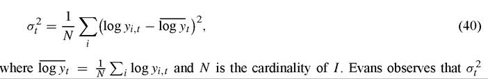
may be represented as a unit root process with a quadratic time trend when there is no cointegration among the series log y_i,_t. This leads Evans to suggest a time-series test of convergence based on unit root tests applied to σ_t². Employing this test, Evans con­cludes that there is convergence to a common trend among 13 industrial countries. One interpretation problem with this analysis is that it allows different countries to possess different deterministic trends in per capita output albeit with the same trend growth rate. Such differences are obviously germane with respect to convergence as an economic concept being consistent, for example, with the club and conditional convergence hy­potheses but not with the unconditional convergence hypothesis. Evans (1997) provides a time series approach to estimating rates of convergence. He shows that OLS applied to Equation (18) yields a consistent estimator of β, and hence the rate of convergence, only if (i) each log y_i,_t - log y_t obeys an AR(1) process having the same AR(1) para­meter lying strictly between 0 and 1; and, (ii) the control variables, X_i and Z_i, account for all cross-country heterogeneity. He argues that neither condition is likely to hold and offers an alternative method of measuring the rate of convergence based on the suppo­sition that log y_i,_t - log y_t follows an AR(q) process with lag polynomial Λ(L). Again, this specification allows countries to follow different parallel balanced growth paths and Evans defines the rate of convergence for economy i as the rate at which log y_i,_t “is ex­pected to revert toward its balanced growth path far in the future”. He shows that, given that it is a real, distinct, positive fraction, the dominant root of the polynomial z^qΛ(z^-1) equals one minus this rate. Evans computes estimates of the convergence rates and their 90% confidence intervals for a sample of 48 countries over the period 1950-90 and for the contiguous US states over the period 1929-91. For the states, about a third of the point estimates are negative and about two-thirds of the confidence intervals contain zero, while for the countries, about half of the point estimates are negative and all but

two of the confidence intervals contain zero. However, in spite of these positive esti­mated average convergence rates of 15.5% and 5.9% respectively, Evans’ analysis fails to yield persuasive evidence in favor of the conditional convergence hypothesis since, in most cases, the hypothesis of a convergence rate of zero cannot be rejected at the 10% level of significance.

Later sections of the chapter will discuss how growth researchers can draw on time series data in other ways. One popular route has been to use panel data, with repeated observations on each country or region. Another method is to use techniques broadly similar to those of event studies in empirical finance, and trace out the consequences of specific events, such as major political or economic reforms. We will consider these approaches in Section 6.3 below.

4.5. Sources of convergence or divergence

Abramovitz (1986), Baumol (1986), DeLong (1988) and many others, both before and since, view convergence as the process of follower countries “catching up” to leader countries by adopting their technologies. Some more recent contributors, such as Barro (1991) and Mankiw, Romer and Weil (1992), adopt the view that convergence is driven by diminishing returns to factors of production.^[338] In the neoclassical model, if each country has access to the same aggregate production function the steady-state is inde­pendent of an economy’s initial capital and labor stocks and hence initial income. In this model, long-run differences in output reflect differences in the determinants of ac­cumulation, not differences in the technology used to combine inputs to produce output. Mankiw (1995, p. 301), for example, argues that for “understanding international expe­rience, the best assumption may be that all countries have access to the same pool of knowledge, but differ by the degree to which they take advantage of this knowledge by investing in physical and human capital”. Even if one relaxes the assumption that coun­tries have access to the same production function, convergence in growth rates can still occur so long as each country’s production function is concave in capital per efficiency unit of labor and each country experiences the same rate of labor-augmenting technical change.

Klenow and Rodriguez-Clare (1997a) challenge this “neoclassical revival” with re­sults suggesting that differences in factor accumulation are, at best, no more important than differences in productivity in explaining the cross-country distribution of output per capita. They find that only about half of the cross-country variation in the 1985 level of output per worker is due to variation in human and physical capital inputs while a mere 10% or so of the variation in growth rates from 1960 to 1985 reflects differences in the growth of these inputs. The differences between the results of Mankiw, Romer and Weil (1992) and the findings of Klenow and Rodriguez-Clare (1997a) in their reex­amination of Mankiw, Romer and Weil have two principal origins. First, citing concerns about the endogeneity of the input quantities, Klenow and Rodriguez-Clare (1997a) es­chew estimation of the capital shares and choose to impute parameters based on the results of other studies. Second, they modify Mankiw, Romer and Weil’s measure of human capital accumulation by supplementing secondary school enrollment rates us­ing data on primary enrollment. This yields a measure of human capital accumulation with less cross-country variation than that used by Mankiw, Romer and Weil. This one modification decreases the relative contribution of cross-country variation in human and physical capital inputs to variation in the 1985 level of output per worker to 40% from the 78% found by Mankiw, Romer and Weil. Prescott (1998) and Hall and Jones (1999) confirm the view that differences in inputs are unable to explain observed differences in output and Easterly and Levine (2001, p. 177) state that “[t]he ‘residual’ (total factor productivity, TFP) rather than factor accumulation accounts for most of the income and growth differences across countries”.

Unlike many authors, who estimate TFP as a residual after assuming a com­mon Cobb-Douglas production function, Henderson and Russell (2004) use a non­parametric production frontier approach (data envelopment analysis) to decompose the 1965 to 1990 growth of labor productivity into (i) shifts in the (common, worldwide) production frontier (technological change); (ii) movements toward (or away from) the frontier (technological catch-up); and (iii) capital accumulation. They find a dominant role for capital accumulation in the growth of the cross-country mean of labor produc­tivity with human and physical capital each accounting for about half of that role.^[339] They also observe that the distribution of labor productivity became more dispersed from 1965 to 1990 and their results suggest that physical and human capital accumula­tion were largely responsible for the increased dispersion.

The results of Henderson and Russell (2004) and those of the previous authors are, however, more consistent than it may seem. Klenow and Rodriguez-Clare (1997a), Hall and Jones (1999) and Barro and Sala-i-Martin (2004) argue that the standard growth accounting decomposition overstates the contribution of capital accumulation to output growth by attributing to capital the effect on output of increases in capital induced by increases in TFP. This effect also applies to Henderson and Russell’s approach and adjusting for it provides some reconciliation of their findings with those of Klenow and Rodriguez-Clare (1997a), Prescott (1998) and Hall and Jones (1999). The standard growth accounting formula attributes a fraction (equal to labor’s share of output) of the growth in output per worker to growth in TFP and a fraction (equal to capital’s share of output) to capital accumulation despite the fact that, in the steady-state, growth in output per worker is entirely due to technological progress [Barro and Sala-i-Martin (2004, pp. 457-460) and Klenow and Rodriguez-Clare (1997a, p. 75, fn. 4)]. The total effect of technological progress on output growth can thus be estimated by dividing labor’s share into the estimated growth rate of TFP Interpreting “capital” broadly, labor’s share is about 1 /3 suggesting that this effect is about three times the rate of growth of TFP Henderson and Russell (2004, Table 5, row (a)) find that, on average, about 90% of the increase in output per worker over the 1965 to 1990 period is attributable to the accumulation of human and physical capital with increases in TFP accounting for the remaining 10%. Applying the adjustment discussed above suggests that technological progress accounts for about 30% of the growth in output per worker over this period while capital accumulation, due to transition dynamics, accounts for the remainder.

As well as determining the relative contributions of inputs and TFP to the cross­country variation in output and output growth, some have studied what features of the cross-country output distribution are explained by the cross-country distributions of in­puts and TFP Henderson and Russell (2004) document the emergence of a second mode in the cross-country distribution of output per worker between 1965 and 1990 and find changes in efficiency (the distance from the world technological frontier) to be largely responsible. A primary role for TFP in determining the shape of the long-run distribu­tion of output per capita is found by Feyrer (2003) who uses Markov transition matrices estimated with data from 90 countries over the period 1970 to 1989 to estimate the ergodic distributions of output per capita, the capital-output ratio, human capital per worker, and TFP. He finds that the long-run distributions of both output per capita and TFP are bimodal while those of both the capital-output ratio and human capital per worker are unimodal. This result, Feyrer observes, has potentially important implica­tions for theoretical modelling of development traps. It suggests that models of multiple equilibria that give rise to equilibrium differences in TFP are more promising than mod­els that emphasize indeterminacy in capital intensity or educational attainment.^[340] It is also consistent with Quah’s (1996c) finding that conditioning on measures of physical and human capital accumulation (and a dummy variable for the African continent) has little effect on the dynamics of the cross-country income distribution.

As discussed in Section 4.3.3, the shapes of ergodic distributions computed from tran­sition matrices estimated with discretized data are not, in general, robust to changes in the way in which the state space is discretized. To avoid these problems, Johnson (2004) extends Feyrer’s analysis using Quah’s (1996c, 1997) continuous state-space methods and finds evidence of bimodality in the long-run distributions of both the capital-output ratio and TFP in addition to that in the long-run distribution of output per capita. This finding is broadly consistent with data produced by a version of the Solow growth model that includes a threshold externality a la Azariadis and Drazen (1990) but may be partly due to the computation of TFP after supposing a Cobb-Douglas production function across countries. Accordingly, some care must be exercised when drawing conclusions from these results.

More generally, in much of the development accounting literature cited above, TFP is measured as a residual under the assumption of a concave worldwide production function. Durlauf and Johnson (1995) present evidence contrary to that assumption and in support of the implied multiple steady states in the growth process. It seems likely that the imposition of a concave production function in this case will tend to exaggerate the measured differences in TFP and so confound inferences about the importance of TFP variation.^[341] While Henderson and Russell (2004)'s approach is nonparametric and free from any assumption of a particular technology per se, it estimates the world technology frontier by fitting a convex cone to data on outputs and inputs. The imposed convexity of the production set prevents the method from discovering any nonconvexities that may exist and, in addition to masking the presence of multiple steady states, convexifying these nonconvexities would tend to overstate the cross-country variation in TFP. The extent to which our current understanding of the relative contributions of variation in inputs and variation in TFP to the observed variation in income levels is influenced by the effects on measured TFP of a misspecified worldwide technology remains an open research question.

Despite these concerns and the differences in the precise estimates found by different researchers, it is clear that cross-country variation in inputs falls short of explaining the observed cross-country variation in output. The result that the TFP residual, a “measure of our ignorance” computed as the ratio of output to some index of inputs, is an impor­tant (perhaps the dominant) source of cross-country differences in long-run economic performance is useful but hardly satisfying and the need for a theory of TFP expressed by Prescott (1998) is well founded. Research such as Acemoglu and Zilibotti (2001) and Caselli and Coleman (2003) are promising contributions to that agenda.

5.