Statistical models of the growth process

While the convergence hypothesis plays a uniquely prominent role in empirical growth studies, it by no means represents the bulk of empirical growth studies. The primary fo­cus of empirical growth papers may be thought of as a general exploration of potential growth determinants.

Section 5.1 discusses the analysis of how specific determinants affect growth. We describe the range of different variables that have appeared in growth regressions and consider alternative methodologies for analyzing growth models in the presence of un­certainty about which regressors should be included to define the “true” growth model. Section 5.2 addresses issues of parameter heterogeneity. The complexity of the growth process and the plethora of new growth theories suggest that the mapping of a given vari­able to growth is likely a function of both observed and unobserved factors; for example, the effect of human capital investment on growth may depend on the strength of prop­erty rights. We explore methods to account for parameter heterogeneity and consider the evidence that has been adduced in support of its presence. Section 5.3 focuses on the analysis of nonlinearities and multiple regimes in the growth process. Endogenous growth theories are often highly nonlinear and can produce multiple steady states in the growth process, both of which have important implications for econometric practice.

5.1. Specifying explanatory variables in growth regressions

In the search for a satisfactory statistical model of growth, the main area of effort has concerned the identification of appropriate variables to include in linear growth regres­sions, this generally amounts to the specification of Z in Equation (18). Appendix B provides a survey of different regressors that have been proposed in the growth literature with associated studies that either represent the first use of the variable or a well known use of the variable.^[342] The table contains 145 different regressors, the vast majority of which have been found to be statistically significant using conventional standards.^[343] One reason why so many alternative growth variables have been identified is due to questions of measurement. For example, a claim that domestic freedom affects growth leaves unanswered how freedom is to be measured. We have therefore organized the body of growth regressors into 43 distinct growth “theories” (by which we mean con­ceptually distinct growth determinants); each of these theories is found to be statistically significant in at least one study.

As Appendix B indicates, the number of growth regressors that have been identi­fied approaches the number of countries available in even the broadest samples. And this regressor list does not consider cases where interactions between variables or non­linear transformations of variables have been included as regressors; both of which are standard ways of introducing nonlinearities into a baseline growth regression. This plethora of potential regressors starkly illustrates one of the fundamental problems with empirical growth research, namely, the absence of any consensus on which growth de­terminants ought to be included in a growth model.

To make this discussion concrete, define S_i as the set of regressors which a researcher always retains in a regression and let R_i denote additional controls in the regression, so that

Notice that the inclusion of a variable in S does not mean the researcher is certain that it influences growth, only that it will be included in all models under consideration. To make this concrete, one can think of an exercise in which one wants to consider the relationship between initial income and growth. A researcher may choose to include initial income and the other Solow growth regressors in every specification of the model, but may in contrast be interested in the effects of different non-Solow growth regressors on inferences about the initial income/growth connection.

If one takes the regressors that comprise R as fixed, then statements about elements of ψ are straightforward. A frequentist approach to inference will compute an estimate of the parameter ψ with an associated distribution that depends on the data generating process; Bayesian approaches will compute a posterior probability density of ψ given the researcher’s prior, the data, and the assumption that the linear model is correctly specified, i.e. the choice of variables in R corresponds to the “true” model. Designating the available data as D and a particular model as m, this posterior may be written as μ(ψ∖D, m).

The basic problem in developing statistical statements either about ψ or μ(ψ ∖D, m) is that there do not exist good theoretical reasons to specify a particular model m. This is not to say that the body of growth theories may not be used to identify candidates for R. Rather, the problem is that growth theories are, using a phrase due to Brock and Durlauf (2001a), open-ended.

One approach to resolving the problem of model uncertainty is based on identifying variables whose empirical importance is robust across different model specifications. This is the idea behind Levine and Renelt’s (1992) use of extreme bounds analysis [Leamer (1983) and Leamer and Leonard (1983)] to assess growth determinants. To see how extreme bounds analysis may be applied to the assessment of robustness of

growth determinants, suppose that one has specified a space of possible models M. For model m, the growth process is

where the subscripts m reflect the model specific nature of the parameters and associated residuals. One can compute ψ_m for every model in M. Motivated by Leamer (1983), Levine and Renelt employ the rule that there is strong evidence that a given regressor in S, call it s_l, robustly affects growth if the sign of the associated regression coefficient ψι_m is constant and the coefficient estimate is statistically significant across all model specifications in M. In this analysis the S vector is composed of a variable of interest and other variables whose presence is held fixed across specifications.

In the Levine and Renelt (1992) analysis, S includes the constant term, initial income, the investment share of GDP, secondary school enrollment rates, and population growth; these variables proxy for those suggested by the Solow model. Models are distinguished by alternative combinations of 1 to 3 variables taken from a set of 7 variables; these correspond to alternative choices of R_im.

) Note that the function /(∙) is allowed to vary across specifications of R. As in Levine and Renelt (1992), Kalaitzidakis, Mamuneas and Stengos conclude that initial income and physical capital investment rates are robust determinants of growth. Unlike Levine and Renelt, they also find that inflation volatility and exchange rate distortions are ro­bust; this is interesting as it is an example where the failure to account for nonlinearity in one set of variables masks the importance of another.

From a decision-theoretic perspective, the extreme bounds approach is a problematic methodology. The basic difficulty, discussed in detail in Brock and Durlauf (2001a) and Brock, Durlauf and West (2003) is that if one is interested in ψ_l because one is consider­ing whether to change s_ig, by one unit, i.e. one is advising country i on a policy change, the extreme bounds standard corresponds to a very risk averse way of responding to model uncertainty. Specifically, suppose that for a policymaker, El(s_i∣, m) represents the expected loss associated with the current policy level in country i. We assume that one is only interested in the case where an increase in the policy raises growth, which means we will assume that it is necessary for ψ_lm > 0 in order to conclude that one should make the change. One can approximate the t-statistic rule, i.e., requiring that the coefficient estimate for sl be statistically significant in order to justify a policy as implying that

where sd(ψ_lm) is the estimate of the standard deviation associated with ψ_lm and the statistical significance level required for the coefficient is assumed to correspond to a t-statistic of 2.

This means that the policymaker must have minimax preferences with respect to model uncertainty, i.e. he will make the policy change only if it yields a positive expected payoff under the least favorable model in the model space. While there are reasons to believe that in practice, individuals assess model uncertainty differently than within- model uncertainty,^[344] the extreme risk aversion embedded in (45) seems hard to justify.

Even when one moves away from decision-theoretic considerations, extreme bounds analysis is somewhat difficult to interpret as a statistical procedure. Hoover and Perez (2004), for example, show that the use of extreme bounds analysis can lead to the con­clusion that many growth determinants are fragile even when they are part of the data generating process. They also find that the procedure has poor power properties in the sense that some regressors that do not matter may spuriously appear to be robust.^[345]

The concern that extreme bounds analysis represents an excessively conservative ap­proach to evaluating empirical results led Sala-i-Martin (1997a, 1997b) to propose a different way to evaluate the robustness of findings. Within a model, suppose there is an evaluative criterion for ψ_m that is used to determine whether the variable s_l matters for the growth process. One example of such a standard is whether or not ψ_lm is sta­tistically significant at some level. Sala-i-Martin first proposes averaging the statistical significance levels via

where S_im is the statistical significance level associated with ψ_m and ω_m is the weight assigned to model m,∑_mω_m = 1. Sala-i-Martin (1997a, 1997b) employs weights determined by the likelihoods of each model as well as employing equal weighting. Second, Sala-i-Martin (1997a, 1997b) proposes examining the percentage of times a variable appears statistically significant with a given sign; a variable whose sign and statistical significance holds across 95% of the different models estimated is regarded as robust. This approach finds that initial income, the investment to GDP ratio and sec­ondary school education are all robust determinants of growth. Sala-i-Martin (1997a,

1997b) extends this analysis to the evaluation of additional variables and finds a num­ber also are robust by his criteria.

While these approaches have the important advantage over extreme bounds analysis of accounting for the informational content of the entire distribution of ψ_m, the pro­cedures do not have any decision-theoretic or conventional statistical justification. We are unaware of any statistical interpretation to averaged significance levels. Further, lit­tle is understood about the statistical properties of these procedures. Hoover and Perez (2004), for example, find that the second Sala-i-Martin procedure has poor size proper­ties, in the sense that “true” growth determinants are still likely to fail to be identified.

Dissatisfaction with extreme bounds analysis and the variants we have described have led some authors to embed the determinants of robust growth regressors in a general model selection context. Hendry and Krolzig (2004) and Hoover and Perez (2004) both employ general-to-specific modeling methodologies generally associated with the re­search program of David Hendry [cf. Hendry (1995)] to select one version of (41) out of the model space. In both papers, the linear model that is selected out of the space of possible models is one where growth is determined by years an economy is open, the rate of equipment investment, a measure of political instability based on the number of coups and revolutions, a measure of the percentage of the population that is Confucian and a measure of the percentage of the population that is Protestant.

Methodologically, these papers in essence employ algorithms which choose a partic­ular regression model from a space of models through comparisons based on a set of statistical tests. The extent to which one finds this approach appealing is a function of the extent to which one is sympathetic to the general methodological foundations of the Hendry research program; we avoid such an extended evaluation here, but simply note that like other general prescriptions the program remains controversial, especially the extent to which it relies on automatic model selection procedures that do not possess a clear decision-theoretic justification. As such, it is somewhat unclear how to evalu­ate the output of the procedure in terms of the objectives of a researcher. That being said, the automated procedures Hendry works with have the important virtue that they can facilitate identifying small sets of models that are well supported by available data. Identification of such models is important, for example, in forecasting, where Hendry’s procedures appear to have a strong track record.

In our judgment, the most promising current approach to accounting for model un­certainty employs model averaging techniques to construct parameter estimates that formally address the dependence of model-specific estimates on a given model. Ex­amples where model averaging has been applied to cross-country growth data include Brock and Durlauf (2001a), Brock, Durlauf and West (2003), Doppelhofer, Miller and Sala-i-Martin (2004), Fernandez, Ley and Steel (2001a) and Masanjala and Papageor- giou (2004). The basic idea in this work is to treat the “true” growth model^[346] as an unobservable variable. In order to account for this variable, each element m in the model space M is associated with a posterior model probability μ(m∖D). By Bayes’ rule,

where μ(D∖m) is the likelihood of the data given the model and μ(m) is the prior model probability. These model probabilities are used to eliminate the dependence of parameter analysis on a specific model. For frequentist estimates, averaging is done across the model-specific estimates ψ_m to produce an estimate ψ via

whereas for the Bayesian context, the dependence of the posterior probability measure of the parameter of interest, μ(ψ ∖D, m) on the model choice is eliminated via standard conditional probability arguments, i.e.

Brock, Durlauf and West (2003) argue that the strategy of constructing posterior prob­abilities that are not model-dependent is the appropriate one when the objective of the statistical exercise is to evaluate alternative policy questions such as whether to change elements of S_i by one unit. Notice that this approach assumes that the goal of the exer­cise is to study a parameter, i.e. ψ, not to identify the best growth model.

Model averaging approaches are still quite new in the growth literature, so many ques­tions exist as to how to implement the procedure. One issue concerns the specification of priors on parameters within a model. Brock and Durlauf (2001a), Brock, Durlauf and West (2003), and Doppelhofer, Miller and Sala-i-Martin (2004) assume a diffuse prior on the model specific coefficients. The advantage of this prior is that, when the errors are normal with known variance, the posterior expected value of ψ, conditional on the data D and model m, is the ordinary least squares estimator ψ_m. The disad­vantage of this approach is that since the diffuse prior on the regression parameters is improper, one has to be careful that the posterior model probabilities associated with the prior are interpretable. For this reason, Doppelhofer, Miller and Sala-i-Martin (2004) eschew reference to their methodology as strictly Bayesian. That being said, so long as the posterior model probabilities include appropriate penalties for model complex­ity [and Brock and Durlauf (2001a), Brock, Durlauf and West (2003), and Doppelhofer, Miller and Sala-i-Martin (2004) all compute posterior model probabilities using BIC ad­justed likelihoods] we do not see any conceptual problem in interpreting this approach as strictly Bayesian. Fernandez, Ley and Steel (2001a) and Masanjala and Papageor- giou (2004) employ proper priors and therefore avoid such concerns.^[347] We are unaware

of any evidence that the choice of prior for the within-model regression coefficients is of great importance in terms of empirical inferences for the growth contexts that have been studied; Masanjala and Papageorgiou (2004) in fact compare results using proper priors with the improper priors we have described and find that the choice of prior is unimportant.

A second unresolved issue concerns the specification of the prior model probabilities μ(m). In the model averaging literature, the general assumption has been to assign equal prior probabilities to all models in M. This prior may be interpreted as assuming that the prior probability that a given variable appears in the “true” model is 0.5 and that the probability that one variable appears in the model is independent of whether others appear. Doppelhofer, Miller and Sala-i-Martin (2004) consider modifications of this prior in which the probability that a given variable appears in the true model is p < 0.5; these alternative probabilities are chosen in order to assign greater weight to more parsimonious growth models, i.e. models in which fewer regressors appear.^[348]

Brock and Durlauf (2001a) and Brock, Durlauf and West (2003) argue against the assumption that the probability that one regressor should appear in a growth model is independent of the inclusion of others. The basic problem with priors that assume independence is analogous to the red bus/blue bus problem in discrete choice theory; namely, some regressors are quite similar to others, e.g., alternative measures of trade openness, whereas other regressors are quite disparate, e.g., geography and institutions. Brock, Durlauf and West (2003) propose a tree structure to organize model uncertainty for linear growth models. First, they argue that growth models suffer from theory un­certainty. Hence, one can identify alternative classes of models based on what growth theories are included. Second, for each specification of a body of theories to be em­bedded, they argue there is specification uncertainty. A given set of theories requires determining whether the theories interact, whether they are subject to threshold effects or other types of nonlinearity, etc. Third, for each theory and model specification, there is measurement uncertainty. The statement that weather affects growth does not specify the relevant empirical proxies, e.g., the number of sunny days, average temperature, etc. Finally, each choice of theory, specification and measurement is argued to suffer from heterogeneity uncertainty, which means that it is unclear which subsets of countries obey a common linear model. Brock, Durlauf and West (2003) argue that one should assign priors that account for the interdependences implied by this structure in assigning model probabilities. Appendix B follows this approach in organizing growth regressors according to theory.

Doppelhofer, Miller and Sala-i-Martin (2004) and Fernandez, Ley and Steel (2001a) employ model averaging methods to identify which growth regressors should be in­cluded in linear growth models. These analyses do not distinguish between variables to be included in all regressions and variables whose inclusion determines alternative mod­els; all variables are pooled and all possible combinations are considered. Doppelhofer, Miller and Sala-i-Martin (2004) working with 31 potential growth determinants, con­clude, weighting prior models so that the expected number of included regressors is 7 (this corresponds to a prior probability of variable inclusion of about 0.25), that four variables have posterior model inclusion probabilities above 0.9: initial income, frac­tion of GDP in mining, number of years the economy has been open,^[349] and fraction of the population following Confucianism. Working with a universe of 41 potential growth determinants, Fernandez, Ley and Steel find that, under the assumption that the prior probability that a given variable appears in the correct growth model is 0.5, four variables have posterior model inclusion probabilities above 0.9: initial income, frac­tion of the population following Confucianism, life expectancy, and rate of equipment investment.

Brock and Durlauf (2001a) and Masanjala and Papageorgiou (2004) employ model averaging to study the reason for the poor growth performance of sub-Saharan Africa. Brock and Durlauf (2001a) reexamine Easterly and Levine’s (1997a) finding that eth­nic heterogeneity helps explain sub-Saharan Africa’s growth problems. This reanalysis finds that the Easterly and Levine (1997a) claim is robust in the sense that ethnic het­erogeneity helps explain why growth in sub-Saharan Africa had stagnated relative to the rest of the world. On the other hand, Brock and Durlauf (2001a) also find that eth­nic heterogeneity does not appear to explain growth patterns in the rest of the world. This leads to the unresolved question of why ethnic heterogeneity has uniquely strong growth effects in sub-Sahran Africa. Masanjala and Papageorgiou (2004) conduct a gen­eral analysis of the determinants of sub-Saharan African growth versus the world as a whole and conclude that the relevant growth variables for Africa are quite different. In particular, variation in sub-Saharan growth is much more closely associated with the share of the economy made up by primary commodities production. They also find, contrary to Doppelhofer, Miller and Sala-i-Martin (2004) that the share of mining in the economy is a robust determinant of growth in Africa but not the world as a whole.

Finally, model averaging has been applied by Brock, Durlauf and West (2003) to analyze the question of how to employ growth regressions to evaluate policy recom­mendations. Specifically, the paper assesses the question of whether a policymaker should favor a reduction of tariffs for sub-Saharan African countries; the analysis as­sumes that the policymaker possesses mean/variance preferences with respect to the effects of changes in current policies with a constant tradeoff of mean against standard deviation of 1 to 2. The analysis finds strong support for a tariff reduction in that it concludes that a policymaker with these preferences should support a tariff reduction for any of the countries in sub-Saharan Africa unless the policymaker has a very strong prior that sub-Saharan African countries obey a distinct linear growth process from the rest of the world. In the case where the policymaker has a strong prior that sub-Saharan Africa is “different” from the rest of the world, there is sufficient uncertainty about the relationship between tariffs and growth for these countries that a change in the rates cannot be justified; the strong prior in essence means that the growth experiences of non-African countries have little effect on the precision of estimates of growth behavior that are constructed using data on sub-Saharan African countries in isolation.

46

5.2. Parameter heterogeneity

From its earliest stages, the use of linear growth models has generated considerable unease with respect to the statistical foundations of the exercise. Arguably, the data for very different countries cannot be seen as realizations associated with a common data generating process (DGP). For econometricians that have been trained to search for a good approximation to a DGP, the modeling assumptions and procedures of the growth literature can look arbitrary. One expression of this concern is captured in a famous remark in Harberger (1987): “What do Thailand, the Dominican Republic, Zimbabwe, Greece, and Bolivia have in common that merits their being put in the same regression analysis?”

Views differ on the extent to which this objection is fundamental. There is general agreement that, when studying growth, it will be difficult to recover a DGP even if one exists. In particular, the prospects for recovering causal effects are clearly weak. Those who are only satisfied with the specification and estimation of a structural model, in which parameters are either ‘deep’ or correspond to precisely defined causal ef­fects within a coherent theoretical framework, will be permanently disappointed.^[350] The growth literature must have a less ambitious goal, namely to investigate whether or not particular hypotheses have any support in the data. In practice, growth researchers are looking for patterns and systematic tendencies that can increase our understanding of the growth process, in combination with historical analysis, case studies, and relevant theoretical models. Another key aim of empirical growth research, which is harder than it looks at first sight, is to communicate the degree of support for any patterns identified by the researcher.

The issue of parameter heterogeneity is essentially that raised by Harberger. Why should we expect disparate countries to lie on a common surface? Clearly this criti­cism could be applied to most empirical work in social science, whether the data points reflect the actions and characteristics of individuals and firms, or the aggregations of their choices that are used in macroeconometrics. What is distinctive about the growth context is not so much the lack of a common surface, as the way in which the sample size limits the scope for addressing the problem. In principle, one response would be to choose a more flexible model that has a stronger chance of being a good approxima­tion to the process generating the data. Yet this can be hard, and an inherently fragile procedure, when the sample is rarely greater than 100 observations.

If parameter heterogeneity is present, the consequences are potentially serious, except in a special case. If a slope parameter varies randomly across units, and is distributed independently of the variables in the regression and the disturbances, the coefficient estimate should be an unbiased estimate of the mean of the parameter. The assumption of independence is not one, however, that may be expected in light of the body of growth theories. For example, when estimating the relationship between growth and investment, the marginal effect of investment will almost certainly be correlated with aspects of the economic environment that should also be included in the regression.

The solution to this general problem is to change the specification in a way that allows greater flexibility in estimation. There are many ways of doing this. One approach is to consider more general functional forms than the canonical Solow regression which for comparison purposes we restate as:

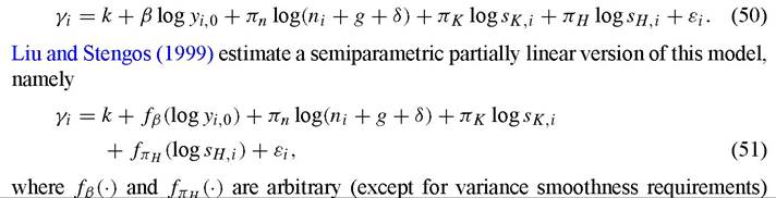
functions. One important finding is that the marginal effect of initial income is only negative when initial per capita income exceeds about $1800. They also find a threshold effect in secondary school enrollment rates (their empirical proxy for log s∏,_i) so the variable is only associated with a positive impact on growth if it exceeds about 15%. Banerjee and Duflo (2003) use this same regression strategy to study nonlinearity in the relationship between changes in inequality and growth; their specification estimates a version of (51) where initial income and human capital investment enter linearly (along with some additional non-Solow variables) but with the addition on the right-hand side of the function fo(G_i^_t — G_i,_t—5) where G_i,_t is the Gini coefficient. Using a panel of 45 countries and 5-year growth averages, their analysis produces an estimate of f_G(-) which has an inverted U shape. One limitation of such studies is that they only allow for nonlinearity for a subset of growth determinants, an assumption that has little theoretical justification and is, from a statistical perspective, ad hoc; of course the approach is more general and less ad hoc then simply assuming linearity as is done in most of the literature.

Durlauf, Kourtellos and Minkin (2001) extend this approach and estimate a version of the augmented Solow model that allows the parameters for each country to vary as functions of initial income, i.e.

This formulation means that each initial income level defines a distinct Solow regres­sion; as such it shifts the focus away from nonlinearity towards parameter heterogeneity, although the model is of course nonlinear in y_i, ₀. This approach reveals considerable pa­rameter heterogeneity especially among the poorer countries. Durlauf, Kourtellos and Minkin (2001) confirm Liu and Stengos (1999) in finding that β(yy_q) is positive for low y_i, ₀ values and negative for higher ones. They also find that π_κ(y_i, ₀) fluctuates greatly over the range of y^₀ values in their sample. This work is extended in Kourtellos (2003a) who finds parameter dependence on initial literacy and initial life expectancy. The varying coefficient approach is also employed in Mamuneas, Savvides and Stengos (2004) who analyze annual measures of total factor productivity for 51 countries. They consider a regression model of TFP in which the coefficient on human capital in the regression is allowed to depend on human capital both in isolation and in conjunction with a measure of trade openness (other coefficients are held constant). Constancy of the human capital coefficient is rejected across a range of specifications.

At a minimum, it generally makes sense for empirical researchers to test for neglected parameter heterogeneity, either using interaction terms or by carrying out diagnos­tic tests. Chesher (1984) showed that White’s information matrix test can be used in this context. For the normal linear model with fixed regressors, Hall (1987) showed that, asymptotically, the information matrix test corresponds to a joint test for het- eroskedasticity and non-normality. Later in the chapter, we discuss how evidence of heteroskedasticity should sometimes be seen as an indicator of misspecification.

Other authors have attempted to employ panel data to identify parameter heterogene­ity without the imposition of a functional relationship between parameters and various observable variables. An important early effort is Canova and Marcet (1995). Defining sγ_t as the logarithm of the ratio of a country’s per capita income to the time t interna­tional aggregate value, Canova and Marcet estimate models of the form

The long-run forecast of s^_t is given by a_i∕(1 — ρ_i) with 1 - ρ_i being the rate of con­vergence towards that value. Canova and Marcet estimate their model using data on the regions of Europe and on 17 Western European countries. Restricting the parameters a_i and ρ_i to be constant across i gives a standard β -convergence test and yields an es­timated annual rate of convergence of approximately 2%. On the other hand, allowing for heterogeneity in these parameters produces a “substantial”, statistically significant, dispersion of the implied long-run s_i,_t forecasts. Moreover, those forecasts are posi­tively correlated with s_i,₀, the initial values of s_i,_t, implying a dependence of long-run outcomes on initial conditions contrary to the convergence hypothesis. For the country­level data, differences in initial conditions explain almost half the cross-sectional varia­tion in long-run forecasts; in contrast, the role of standard control variables such as rates of physical and human capital accumulation and government spending shares is minor. The latter finding must be tempered by the fact that the sample variation in these con­trols is less than that in Barro (1991) or Mankiw, Romer and Weil (1992), for example.

A similar approach is taken by Maddala and Wu (2000) who consider models of the form

log yi,t = αi + ρi logyi,t-1 + ui,t,

(54)

which is of course very similar to the model analyzed by Canova and Marcet (1995). Employing shrinkage estimators for α_i and ρ_i, they conclude that convergence rates, measured as β_i = - log ρ_i exhibit substantial heterogeneity.

5.3. Nonlinearity and multiple regimes

In this section we discuss several papers that have attempted to disentangle the roles of heterogeneous structural characteristics and initial conditions in determining growth performance. These studies employ a wide variety of statistical methods in attempting to identify how initial conditions affect growth. Despite this, there is substantial con­gruence in the conclusions of these papers as these studies each provide evidence of the existence of convergence clubs even after accounting for variation in structural charac­teristics.

An early contribution to this literature is Durlauf and Johnson (1995) who use classi­fication and regression tree (CART) methods to search for nonlinearities in the growth process as implied by the existence of convergence clubs.^[351] The CART procedure iden­tifies subgroups of countries that obey a common linear growth model based on the Solow variables. These subgroups are identified by initial income and literacy, a typ­ical subgroup l is defined by countries whose initial income lies within the interval d_ly ≤ y_i,0 < Cy and whose literacy rate L_i lies in the interval d_lL ≤ L_i < ¾_l. The number of subgroups and the boundaries for the variable intervals that define them are chosen by an algorithm that trades off model complexity (i.e. the number of sub­groups) and goodness of fit. Because the procedure sequentially splits the data into finer and finer subgroups, it gives the data a tree structure.

Durlauf and Johnson (1995) also test the null hypothesis of a common growth regime against the alternative hypothesis of a growth process with multiple regimes in which economies with similar initial conditions tend to converge to one another. Using in­come per capita and the literacy rate (as a proxy for human capital) to measure the initial level of development and, using the same cross-country data set as Mankiw, Romer and Weil, Durlauf and Johnson reject the single regime model required for global convergence. That is, even after controlling for the structural heterogeneity implied by Mankiw, Romer and Weil’s augmented version of the Solow model, there is a role for initial conditions in explaining variation in cross-country growth behavior.

Durlauf and Johnson’s (1995) findings of multiple convergence clubs appear to be reinforced by subsequent research. Papageorgiou and Masanjala (2004) note that one possible source for Durlauf and Johnson’s findings may occur due to the misspec­ification of the aggregate production function. As observed in Section 2, the linear representation of the Solow model represents an approximation around the steady-state when the aggregate production function is Cobb-Douglas. Papageorgiou and Masan- jala estimate a version of the Solow model based on a constant elasticity of substitution (CES) production function rather than the Cobb-Douglas, following findings in Duffy and Papageorgiou (2000). They then examine the question of whether or not Durlauf and Johnson’s multiple regimes remain under the CES specification. Using Hansen’s (2000) approach to sample splitting and threshold estimation, they find statistically sig­nificant evidence of thresholds in the data. The sample splits they estimate divide the data in four distinct growth regimes and are broadly consistent with those found by Durlauf and Johnson.^[352]

These findings are extended in recent work due to Tan (2004) who employs a pro­cedure known as GUIDE (generalized, unbiased interaction detection and estimation) to identify subgroups of countries which obey a common growth model.^[353] Relative to CART, the GUIDE algorithm has two advantages: (1) the algorithm explicitly looks for interactions between explanatory variables when identifying splits, and (2) some within model testing supplements the penalties for model complexity and thereby reduces the tendency for CART procedures to produce an excessive number of splits in finite sam­ples. Tan (2004) finds strong evidence that measures of institutional quality and ethnic fractionalization define convergence clubs across a wide range of countries. He also finds weaker evidence that geography distinguishes the growth process for sub-Saharan Africa from the rest of the world.

Further research has corroborated the evidence of multiple regimes using alternative statistical methods. One approach that has proved useful is based on projection pursuit methods.^[354] Desdoigts (1999) uses these methods in an attempt to separate the roles of microeconomic heterogeneity and initial conditions in the growth experiences of a group of countries and identifies groups of countries with relatively homogeneous growth experiences based on data about the characteristics and initial conditions of each country. The idea of projection pursuit is to find the orthogonal projections of the data into low-dimensional spaces that best display some interesting feature of the data. A well-known special case of projection pursuit is principal components analysis. In principal components analysis, one takes only as many components as are neces­sary to account for “most” of the variation in the data. Similarly, in projection pursuit one should only consider as many dimensions as needed to account for “most” of the clustering in the data.

Desdoigts finds several interesting clusters. The first is the OECD countries. The two projections identifying this cluster put most of their weight on the primary and sec­ondary school enrollment rates, the 1960 income gap and the rate of growth in the labor force. The prominence of variables that Desdoigts argues are proxies for initial condi­tions among those defining the projections leads him to conclude that initial conditions are more important in defining this cluster than are other country characteristics. Reap­plication of the clustering method to the remaining (non-OECD) countries yields three sub-clusters that can be described as Africa, Southeast Asia, and Latin America. Here the projections put most weight on government consumption, the secondary school en­rollment rate and investment in electrical machinery and transportation equipment. Most of these variables are argued to proxy for structural characteristics of the economies, suggesting that they, rather than initial conditions, are responsible for the differences in growth experiences across the three geographic sub-clusters. Nevertheless, this ap­proach relies on the judgment of the researcher in determining which variables proxy for initial conditions and which proxy for structural characteristics.

Further evidence of the utility of projection pursuit methods may be found in Kourtellos (2003b). Unlike Desdoigts, Kourtellos (2003b) uses projection pursuit to construct models of the growth process. Formally, he estimates models of the form

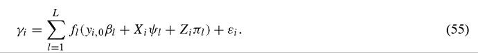
Each element in the summation represents a distinct projection. Kourtellos uncovers evidence of two steady-states, one for low initial income and low initial human capital countries.

A third approach to multiple regimes is employed by Bloom, Canning and Sevilla (2003) based on the observation that if long-run outcomes are determined by funda­mental forces alone, the relationship between exogenous variables and income levels ought to be unique. If initial conditions play a role there will be multiple relationships - one for each basin of attraction defined by initial conditions. If there are two (stochas­tic) steady states, and large shocks are sufficiently infrequent,⁵² the system will, under suitable regularity conditions, exhibit an invariant probability measure that can be de­scribed by a “reduced form” model in which the long-run behavior of log y^_t depends only on the exogenous variables, m_i, such as

⁵² The assumed rarity of large shocks implies that movements between basins of attraction of each of the steady states are sufficiently infrequent that they can be ignored in estimation. This assumption is consistent with, for example, Bianchi’s (1997) finding of very little mobility in the cross-country income distribution.

and

where uyp and u₂,pt are independent, zero-mean deviations from the steady-state log means log yf (m_i) and log y₂(m_i) respectively, and p(m_i) is the probability that coun­try i is in the basin of attraction of the first of the two steady states. From the perspective of the econometrician, log yp thus obeys a mixture process. The two steady states asso­ciated with (56) and (57) are possibly interpretable as a low-income regime or poverty trap and as a high-income or perpetual growth regime respectively. Bloom, Canning and Sevilla estimate a linear version of this model using 1985 income data from 152 countries with the absolute value of the latitude of the (approximate) center of each country as the fundamental exogenous variable. They are able to reject the null hypoth­esis of a single regime model in favor of the alternative of a model with two regimes - a high-level (manufacturing and services) steady state in which income is independent of latitude and a low-level (agricultural) steady-state in which income depends on latitude (presumably through its influence on climate). In addition, the probability of being in the high-level steady state is found to rise with latitude.

A final approach to multiple regimes is due to Canova (2004) who introduces a proce­dure for panel data that estimates the number of groups and the assignment of countries or regions to these groups, drawing on Bayesian ideas. This approach has the impor­tant feature that it allows for parameter heterogeneity across countries within a given subgroup. The researcher can order the countries or regions by various criteria (for ex­ample, output per capita in the pre-sample period) and the estimation procedure then chooses break points and group membership in such a way that the predictive ability of the overall model is maximized. This approach is applied to autoregressive models of per capita output as in Equation (54) above.

Using data on per capita income data in the regions of Europe, Canova (2004) finds that ordering the data by initial income maximizes the marginal likelihood of the model and breaks the data into 4 clusters. The estimated mean steady-states for each group are significantly different from each other implying that the groups are convergence clubs. The differences in the means are also economically important with the lowest and highest being 45% and 115% of the overall average respectively. Canova finds little across-group mobility especially among those regions that are initially poor. Using data on per capita income in the OECD countries, two clusters are found and, again, initial per capita income is the preferred ordering variable. The estimated model parameters imply an “economically large” long-run difference in the average incomes of countries in the two groups with little mobility between them.

In assessing these analyses, it is important to recognize an identification problem in attempting to link evidence of multiple growth regimes to particular theoretical growth models. As argued in Durlauf and Johnson (1995), this identification problem relates to whether evidence of multiple regimes represents evidence of multiple steady-states as opposed to nonlinearity in the growth process.

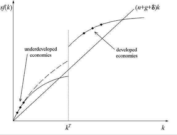
Figure 8. Nonlinearity versus multiple steady-states.

To see why this is so, suppose that one has identified two sets of countries that obey separate growth regimes with regime membership determined by a country's initial cap­ital stock, i.e. there exists a capital threshold k^τ that divides the two groups of countries. An example of this can be seen in Figure 8. Clearly, the two sets of countries do not obey a common linear model but it is not clear whether or not multiple steady-states exist. The output behavior of low capital countries is compatible with either the solid or dashed curve in the lower part of the figure, but only the solid curve produces multiple steady-states. The identification problem stems from the fact that one does not have ob­servations that allow one to distinguish differences in the long-run behavior of countries that start with capital stocks in the vicinity of k^τ. This argument does not depend on growth regimes determined by the capital stock but it does depend on whether or not the variable or variables that define the regimes are growing over time, as would occur for initial income or initial literacy. For growing variables, the possibility exists that countries currently associated with low levels of the variables will in the future exhibit behaviors that are similar to those countries which are currently associated with high levels of the variables.

How might evidence of multiple steady-states be established? One possibility is via the use of structural models in empirical analysis. While this has not been done econo- metrically, Graham and Temple (2003) follow this strategy and calibrate a two-sector general equilibrium model with increasing returns to scale in nonagricultural produc­tion. Their empirically motivated choice of calibration parameters produces a model which implies that some countries are in a low-output equilibrium. Another possibility is to exploit time series variation in a single country to identify the presence of jumps from one equilibrium or steady state to another.

6.