7. Non-neutral differences in technology
7.1. Basic concepts and qualitative results
In all of the previous sections we have assumed that all differences in efficiency across countries are TFP differences, as summarized by the multiplicative factor A.
This im-64
See also Chanda and Dalgaard (2003) for another contribution that argues for a large role of agriculture.
plies that we view differences in efficiency as factor neutral: some countries simply use all of their inputs more efficiently than others. This is of course a restriction on the set of possible efficiency differences. Caselli and Coleman (2005) have begun exploring a more general view, that allows for the possibility that differences in technology show up as differences in the efficiency with which specific factors - as opposed to all factors proportionally - are used, or even that some countries use some factors more efficiently, and some less efficiently, than others. In other words, a more general view of technology differences where such differences are not factor neutral.65
Extending the development-accounting exercise to allow for factor non neutrality in efficiency differences is the object of this section. While Caselli and Coleman consider a three-factor production function (capital, skilled labor, and unskilled labor), here I will stick to the two-factor world (human and physical capital) of the rest of the chapter. The first step we need to take to proceed in this direction is to replace the Cobb-Douglas restriction - which implicitly rules out non-neutrality - with a more general production function where non-neutral differences can be contemplated. The simplest such generalization is provided by the CES formula:

In (17) Ak and Ah are the efficiency units delivered by one unit of physical capital and one unit of quality-adjusted labor, respectively.
If Ak is higher in one country than in another, we say that the former country uses capital more efficiently. If Ah is greater, the country uses human capital more efficiently. The parameters σ and α are constant across countries. σ governs the ease of substitution between physical and human capital. The elasticity of substitution is
The Cobb-Douglas case of the previous sections of the paper emerges as a limit for σ approaching 0 (η approaching 1). In this case, total factor productivity A converges to

In the factor-neutral world explored so far in this chapter, making inference about efficiency differences across countries is a simple matter of solving one equation in one unknown. Inference on non neutral differences is a bit more challenging, as Equation (17) has two unknowns: Ak and Ah. The issue, then, is to find a suitable second equation. As in Caselli and Coleman (2005), to do so I assume that factor markets are everywhere competitive. Then, if r is the user cost of capital, and if w is the market
price of a unit of human capital, the following equations will hold:

Given values of α and σ, and data on y,k,h,r, and w, these two equations can be solved for the two unknowns Ak and Ah.[420]
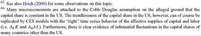
Rearranging Equations (18) we find the following formulas for the factor-specific efficiency levels
where Sk and Sh are the shares of physical and human capital in income, respectively.
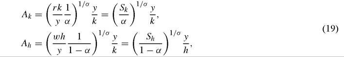
To see what these equations tell us about the way technology differs across countries it is useful to start from the case where factor shares are constant across countries, i.e. Sk and Sh are invariant parameters. Note that this is the assumption we have maintained so far throughout the paper, where we have set Sk to α (and consequently Sh to 1 — α). Under this assumption, these equations have very intuitive implications: a high output-capital ratio implies that capital is used efficiently, and the same for human capital.Figure 18 plots the output-capital ratio y/k against the log of per-capita income, and Figure 19 does the same for the output-human capital ratio, y/h. As is well known, the output-capital ratio is decreasing in income. The output-human capital ratio, instead, is increasing. Hence, if we continue to assume that factor shares are constant across countries, but we allow for non-neutrality in technology differences, we reach the startling conclusion that rich countries use human capital more efficiently than poor countries, but they use physical capital less efficiently.[421]
Consider now relaxing the assumption of constant factor shares. Clearly our conclusions would be unchanged if the factor shares, while not constant, were not systematically related with income. Our knowledge of cross-country patterns in factor shares is somewhat limited. The only thing we are quite sure of is that in the US this share has historically been rather stable, at around 1/3. When it comes to cross-country comparisons, however, we are on shakier ground. Traditionally, the capital share - as measured in the national accounts - is calculated as a residual after employee compensation has been taken out. With this method, Sk is generally found to be higher in poor countries
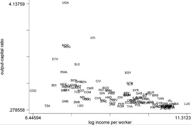
Figure 18. Distributionof y/k.
Figure 19.
Distributionof y/h.
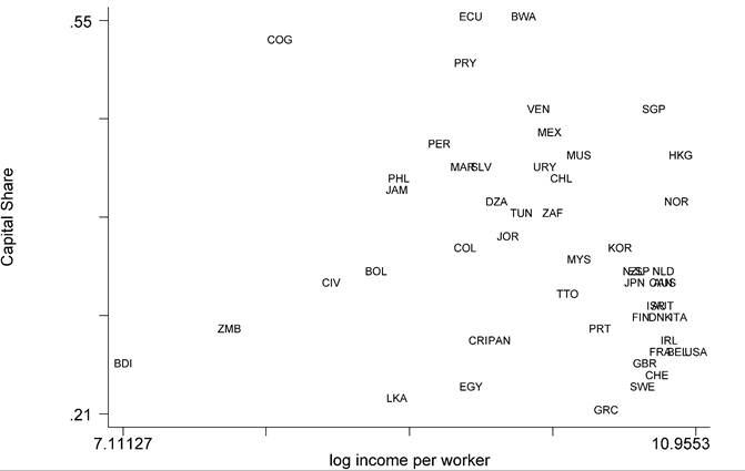
Figure 20. Distributionof Sk.
than in rich countries. Recently, however, Gollin (2002), and Bernanke and Gurkaynak (2001) have convincingly criticized the construction of the traditional estimates of the capital share, and have provided revised estimates that - among other things - attempt to include the labor component of self-employment income in the labor share. These estimates are plotted in Figure 20.[422] Figure 20 shows essentially no systematic pattern of cross-country variation in capital shares. This supports our preliminary finding: the efficiency of capital is higher in poor countries, and the efficiency of (quality adjusted) labor is higher in rich ones!
Unfortunately, the data set on capital shares is small - only 54 observations - and developed economies are over-represented. Furthermore, many untested assumptions have been used to develop these estimates. Hence, the conclusion that capital shares are not systematically related to labor productivity is not iron tight. What would it take then to reverse the startling result that poor countries are more efficient users of capital?
If factor shares vary systematically with per-worker income, then it becomes critical to know what is the elasticity of substitution η = 1/(1 — σ). Suppose that Sk is higher in rich countries. If σ > 0 (i.e. η > 1, or capital and human capital are good substitutes
Table 6
Predicted correlations between Ak and y, and Ah and y
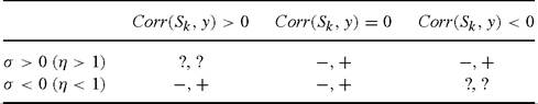
relative to the Cobb-Douglas case), then Ak may conceivably become increasing in income [if (Sk)γ∕σ grows “fastef’ than y/k falls]. In this case, however, since Sh = 1 - Sk the result on Ah could also possibly be overturned.
If σ < 0 (or η < 1) the results from the constant-share case would be reinforced. Symmetrically, if Sk is decreasing in income, the negative (positive) correlation between Ak (Ah) and y would be reinforced for σ > 0(η > 1), and weakened (and possibly overturned) if σ < 0(η < 1). These observations are summarized in Table 6. Each cell of the table lists the predicted sign (positive, negative, or ambiguous) for the correlation between Ak and y (first term) and between Ah and y (second term), conditional on the observed patterns of y/k and y/h, under various assumptions on σ, and on the correlation between Sk and y.The intuition for the way observed factor shares modify our predictions on crosscountry efficiency patterns is simple. If σ > 0 the two factors are good substitutes. Because the two factors are good substitutes, it makes sense to try to increase the usage of the most efficient factor. Hence, when σ > 0 demand will concentrate on the factor with high efficiency, leading to a high share in income for this factor. Conversely, then, with σ > 0, when we observe a high income share for factor x we can infer that this factor is efficient. On the other hand, if σ < 0 the two factors are poor substitutes. In this case, allocative efficiency calls for boosting the overall efficiency units provided by the low-efficiency factor. This increases the income share of this factor. Hence, with σ < 0, a high income share for factor x signals that this factor is used inefficiently.
In sum, skepticism about the greater capital efficiency of poor countries is authorized if one believes that there is a strong positive correlation between Sk and income and η > 1; or if one believes that there is a strong negative correlation between Sk and y and η < 1. We have seen what the data say about Sk (no correlation): what about η?
Hamermesh (1993) provides an exhaustive survey, featuring firm, industry, and country-level studies, both cross-sectional and time series.
Unfortunately, he reports a dismayingly wide range of estimates, both greater and less than one. To my knowledge, additional recent contributions have not helped narrowing down the region in which η may fall.[423] Since published estimates of η are neither stable, nor reliable, one could, perhaps, turn to theoretical considerations. There is of course a tradition of arguing thatTable 7
Regressions of log(Afc) and log(A⅛) on log(y)
| Dep. var. | η = 0.1 | η = 0.5 | η = 0.9 | η = 1.1 | η = 1.5 | η=2 | η = 50 |
| log(Afc) | —0.32 | —0.027 | 0.14 | —0.89 | —0.48 | —0.43 | —0.37 |
| (6.2) | (4.28) | (0.39) | (1.99) | (3.58) | (4.38) | (5.59) | |
| log(As) | 0.80 | 0.74 | 0.21 | 1.53 | 1.00 | 0.94 | 0.87 |
| (28.06) | (17.55) | (.88) | (5.36) | (12.88) | (17.37) | (25.57) |
long-run elasticities are higher than short-run ones, and macro-economic higher than micro-economic. Ventura (1997) is a particularly convincing recent example. For our purposes it clearly seems appropriate to focus on a long-run, aggregate interpretation of the elasticity. However, it is not clear that even in this case these arguments put a lower bound on η: even accepting that it is higher than a microeconomic, short-run elasticity, does not necessarily imply that it is, say, greater than 1.
For the countries with available data, we can actually compute the implied values of Afc and As from Equation (19) for different values of the elasticity of substitution η. For each of these implied set of estimates, in Table 7 we report the coefficients of regressions of log(Afc) and log(Ah) on log(y) (t-statistics in parenthesis).71 The results from the table confirm that the available data is mostly consistent with the situation in the middle column of Table 6: for most values of η, rich countries seem to use capital less efficiently than poor ones. The only exception is for η = 0.9, where Afc is weakly and insignificantly positively related to income. This is not surprising, since η = 0.9 is “almost” Cobb-Douglas, and in this limiting case Afc and Ah are not independently identifiable. The coefficients are also sizable, with a 10 percent increase in income per worker being associated with up to a 9 percent decline in Afc, and even larger increases in Ah.
Everything considered, the result that poor countries use capital more efficiently than rich ones seems surprisingly robust, particularly because very little structure is imposed on the data to reach this conclusion. Needless to say, it is also rather stunning - especially if one is used to think about the world in TFP (factor neutral) terms. However, a possible theoretical explanation is readily available.
will be mis-measured, perhaps wildly. I believe this may indeed be the reason why estimates of η are so unstable. I think this point is implicit in the analysis of Diamond, McFadden and Rodriguez (1978). If the induced measurement error is random, it seems the bias in the estimate of η should be upwards. Intuitively, observations with very different input combinations will appear to have similar output levels, something that is consistent with a high elasticity of substitution. However, if the As vary systematically, the bias could also be downward. Suppose, for example, that Ax and x are positively correlated across observations. Then the data will tend to understate the true variation in effective input, so that less substitutability will appear to be required to explain the observed variation in output.
71 In these regressions there are 53 observations for log(Afc) and 50 for log(A⅛). Also notice that, from Equations (19), the As are identified up to the common multiplicative constants α1 1σ and (1 — α)11/.
Caselli and Coleman (2005) find somewhat analogous evidence that poor countries use unskilled labor more efficiently than rich countries - while rich countries use skilled labor more efficiently. To explain this finding they develop a simple model of appropriate technology, in which countries face a menu of technology choices. The choice of technology is not neutral, in that different technologies augment different inputs differently. One key result is that which technology is chosen by each country depends on the elasticity of substitution between inputs. If the elasticity of substitution is greater than 1, the appropriate technology augments the abundant factor relatively more, while if the elasticity is less than 1, it is appropriate to choose a technology that augments the scarce factor relatively more. Since the elasticity of substitution between skilled and unskilled workers is commonly deemed to be in the neighborhood of 1.4, and rich countries are abundant in skilled labor, this explains why they would choose skilled-labor augmenting technologies, while poor countries choose unskilled-labor augmenting technologies.
Returning now to the new result here that poor countries use physical capital more efficiently - and human capital less efficiently - than rich countries, and recalling that poor countries are relatively abundant in human capital, we can use the same theoretical explanation if we are willing to assume that the elasticity of substitution between capital and (quality-adjusted) labor is less than 1; an assumption that - as we have seen - cannot be ruled out based on the available evidence. In sum, with a high elasticity of substitution between skilled and unskilled labor, and a low elasticity of substitution between capital and the labor aggregate, an appropriate technology model can explain the joint patterns of cross-country choice of the efficiency of capital, skilled labor, and unskilled labor.72
7.2. Development accounting with non-neutral differences
Development accounting asks how the observed distribution of GDP per worker compares to the distribution that would obtain in the counterfactual case that all countries had the same technology. As is clear from Equation (17), we are again in the situation in which - unlike in the simple TFP framework - the answer to this question will not be insensitive to which particular pair of values of Ak and Ah are plugged in. As we did in the previous subsection, and for the same reasons, I choose as the benchmark country the USA. Hence, I first compute the US Ak and Ah from Equations (19), and then I plug these numbers in Equation (17) for each country, and obtain measures of success of a model where all countries use the same (US) technology.73
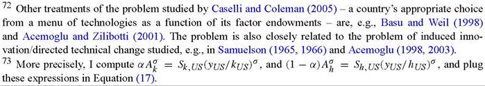

Figure 21. Success with non-neutral technology differences.
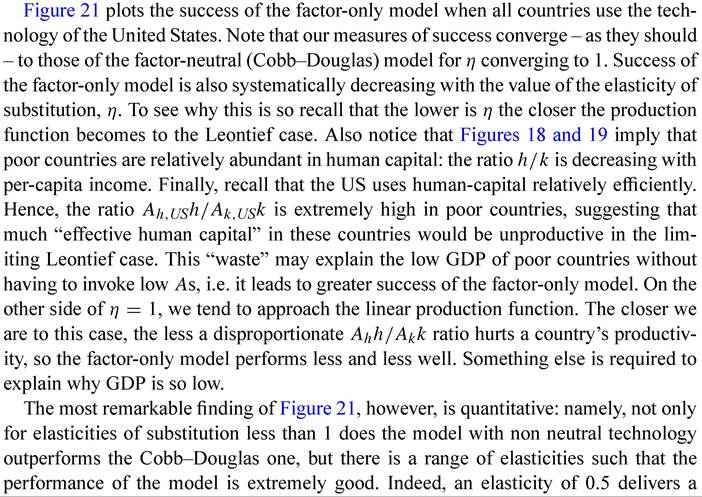
perfect fit for the factor-only model! This is remarkable because an elasticity of 0.5 - given our current state of knowledge - is not particularly implausible.[424]
One could object to the exercise we just reported that the counter-factual choice of technology - all countries using the US technology - is not sensible. For, we know from the previous section that - assuming our factor share data to be dependable - countries are observed to use technologies that cannot be ranked: some technologies boost the productivity of physical capital, some others of human capital. Therefore, one may speculate that - given the choice - poor countries would not necessarily choose to use the US technology. Instead, they would choose the technology most appropriate given their factor endowments.
In order to address this point, we now treat the observed (Ak, Ah) combinations from the previous sub-section as a “menu” of available technologies. One could think of this menu as a summary of the world’s technical knowledge, each observed (Ak, Ah) pair being a particular blueprint to generate output from physical and human capital. I then re-interpret the counter-factual of no technology differences as one where all countries have access to the same menu of technologies; ask what technology from this menu would each country choose; and compute the counter-factual world income distribution when all countries choose their appropriate technology (from the set of available ones). The appropriate technology is the output-maximizing one.[425]
The results from this alternative counter-factual experiment are plotted in Figure 22. Here, foreach value of η, I have computed from Equations (19) the implied values of Ak and Ah for each country with complete data - including data on the factor shares Sk and Sh. This gave us 50 “observed” technologies. For each country in our 94-country sample, then, I have “chosen” from this menu of 50 the appropriate technology, and I have computed success under the assumption that each country uses this output-maximizing choice. As can be seen, the results preserve the broad qualitative features of those of Figure 21, but quantitatively the factor-only model does much less well. In particular (almost), complete success only occurs if the technology is Leontief.
The intuition for this change in results is simple. Given the observed wide disparity in factor proportions, when countries can choose their technology appropriately they will in general choose different (Ak, Ah) combinations. In particular, few poor countries will find it optimal to use the technology observed in the USA. Indeed, countries with unfavorable factor endowments will be able to partially remedy by choosing technology appropriately. Hence, factor endowments do not have as much explanatory power for income differences as they do when all countries are forced to use the same (US) technology.
Even when countries choose technology, however, the measures of success are very sensitive to the choice of the elasticity of substitution: if the elasticity of substitution is
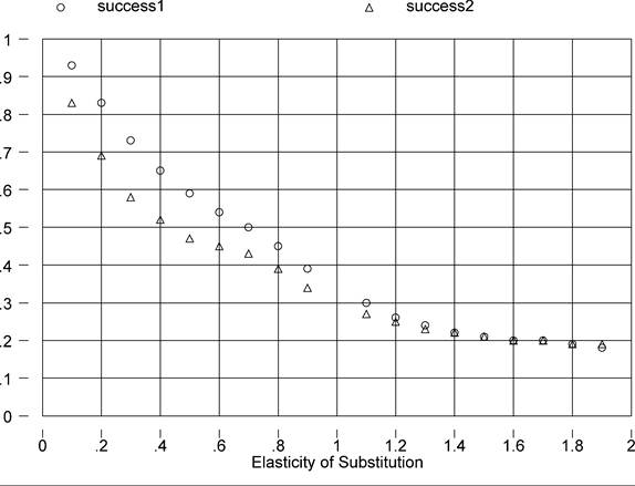
Figure 22. Success with non-neutral but appropriate technology.
low factor endowments can explain a substantially larger share of income differences than in the Cobb-Douglas case (and if it is high a substantially smaller share). It is therefore appropriate to conclude that the Cobb-Douglas assumption is a very sensitive one for development accounting, and that seemingly innocuous generalizations of this assumption - such as the CES formulation employed in this section - can lead to radical changes in results.
8.