Sectorial differences in TFP

Up to here in this chapter I have treated a country’s GDP as if it was produced in a single sector, i.e. as if GDP measured the physical output of a homogeneous good. The basic message has been that it is impossible to explain cross-country differences in income without admitting a large role for differences in TFP.

6.1. Industry studies

There is a tradition of productivity comparisons at the industry, or even at the firm, level. Particularly illustrative of the advantages of this approach are a series of reports published by the McKinsey Global Institute. These studies focus on painstaking com­parisons of the production functions (broadly construed) of narrowly defined industries (from automobile, to beer, to retail banking) in a few industrialized economies (mostly US, Japan, Germany, and the UK). Baily and Solow (2001) present a thoughtful survey of the achievements, as well as the shortcomings, of these studies (as well as extensive references).^[418]

Briefly, even within narrowly defined industries, and even among countries at very similar levels of development, total factor productivity presents remarkable variation. A similar conclusion, for somewhat more aggregated manufacturing industries (but more countries), is reached by Harrigan (1997, 1999).

Besides confirming that TFP differences exist also at the industry level, the McKinsey researchers are often also able to shed some tentative light on their sources. In particular, they highlight differences in working practices, and they are sometimes also able to link inefficient practices to the regulatory environment. In general, the studies point to a link between the degree of competition domestic producers are exposed to (as affected by the amount of regulation), and the efficiency with which they organize their labor input. This is of course an important, and plausible, finding. Further support for this view comes from the work of Schmitz (2001) on the North-American iron-ore industry, which shows convincingly that the efficiency of labor practices is very responsive to the degree of product-market competition.^[419]

6.2. The role of agriculture

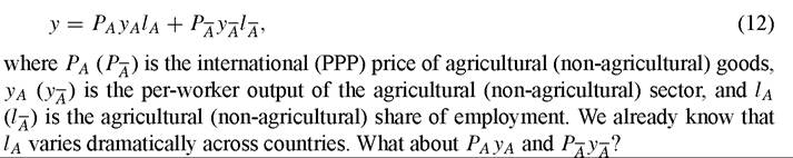
As mentioned, existing cross-country comparisons of sectorial TFP tend to be limited to small sets of developed countries. The goal of this section is therefore to provide a rough, preliminary assessment of the sectorial-composition interpretation of TFP dif­ferences that extends to developing countries as well. In particular, I will focus on an agriculture-nonagriculture split of GDP. The main reason for looking at this particular breakdown is easily inferred from Figure 15: in the poorest countries of the world virtu­ally everyone works in agriculture, and in the richest virtually nobody does. It is obvious that this is the most important source of variation in the composition of GDP around the World. Another reason for focusing on agriculture is that I have no PPP output data for other sectors.

The main purpose of this section, then, is to assess the hypothesis that (i) agriculture is an intrinsically low TFP sector, and (ii) poor countries' low aggregate TFP is due

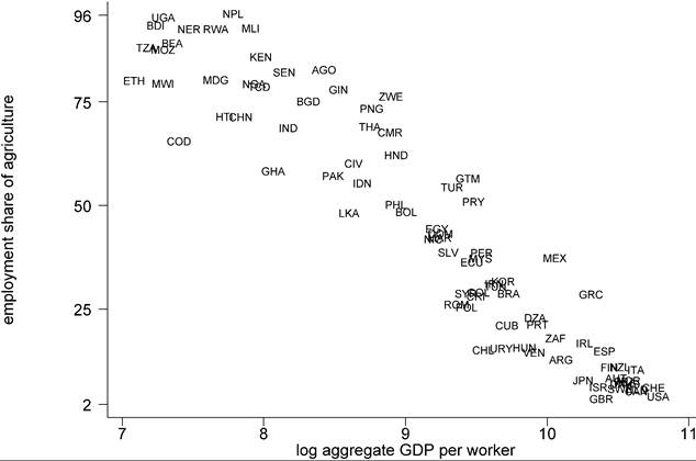
Figure 15. The importance of agriculture.

the source of the productivity differences boils down to the fact that each English worker was willing to tend to a much larger number of machines. In low-productivity countries workers were idle most of the time. Why this was so remains a bit of a mystery, and one should be cautious in assuming that this finding would still hold up one century later. Nevertheless, Clark's findings reinforce the case that labor practices may be an important source of observed differences in productivity.

⁵³ Some of the classics are Fisher (1945), Clark (1940), Rostow (1960), Nurkse (1953), Lewis (1954), Kuznets (1966), and Jorgenson (1961).

in substantial measure to their high shares of agriculture. In this subsection, however, I start by taking a preliminary (and perhaps somewhat digressive) look at basic data on agricultural GDPs, non-agricultural GDPs, and agricultural labor shares. What we find should provide further motivation for asking the development-accounting question with disaggregated data.

I begin by writing per-worker GDP in PPP as

The Food and Agriculture Organization (FAO) has collected and published cross­country data on producer prices in agriculture for a large number of countries between 1970 and 1990 [Rao (1993), see also Restuccia, Yang and Zhu (2003)]. This permits the construction of PPP exchange rates for agriculture, and therefore of PPP compar­isons of agricultural output. Going even further, the FAO researchers also assembled some data on agricultural inputs for the year 1985, and this allowed them to generate a cross-section of PPP agricultural GDPs.

A difficulty that needs to be addressed, however, is that the FAO numbers for PPP agricultural GDP do not directly map into the quantity PAyA in Equation (12). The reason is as follows. The FAO PPP GDPs aggregate the quantities of the various agricul­tural products by a set of “international prices”, that are essentially weighted averages of each country’s prices. The same is done in the PWT for all goods and services. How­ever, the two systems use a different normalization for the international prices - i.e. they have the same relative prices of agricultural products but different absolute levels. Hence, the PPP agricultural value-added coming from the FAO data set cannot sim­ply be plugged into Equation (12) with PWT aggregate value added on the left hand side.⁵⁴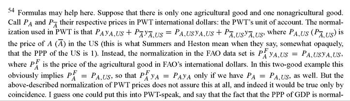

I try to solve this problem as follows. It is well known that - because they are quantity-weighted - international-dollar relative prices in the PWT closely resemble rich-country, and especially US, relative prices [Hill (2000)]. Hence, for the US, we should have

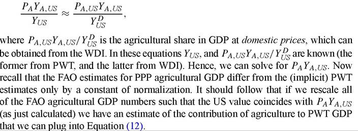
As already pointed out by Restuccia, Yang and Zhu (2003), the most striking feature of the FAO data is that variation in agricultural value-added per worker (in PPP) dwarfs the variation in aggregate value-added per worker. In the largest sample with data on both agricultural and aggregate GDP per worker (80 countries) the inter-percentile range in agricultural GDP is 45 and the log-variance is 2.15.

Subtracting real agricultural GDP from aggregate GDP, it is also possible to back out non-agricultural value-added per worker.⁵⁶ The (not surprising but nonetheless) very important finding is that differences in labor productivity in the non-agricultural sector are much smaller than differences in aggregate labor productivity (and, a fortiori, in agricultural labor productivity). The inter-percentile range is only 4.16 (compared with 22 for aggregate GDP and 45 for agriculture) and the log-variance is 0.33 (compared with 1.18 and 2.15). Figure 17 plots non-agricultural value-added per worker against aggregate value-added per-worker. Comparison of Figures 16 and 17 shows that labor productivity is generally higher outside than inside agriculture, and this is much more true for developing countries, an observation previously made by Gollin, Parente and Rogerson (2000).⁵⁷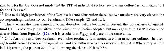

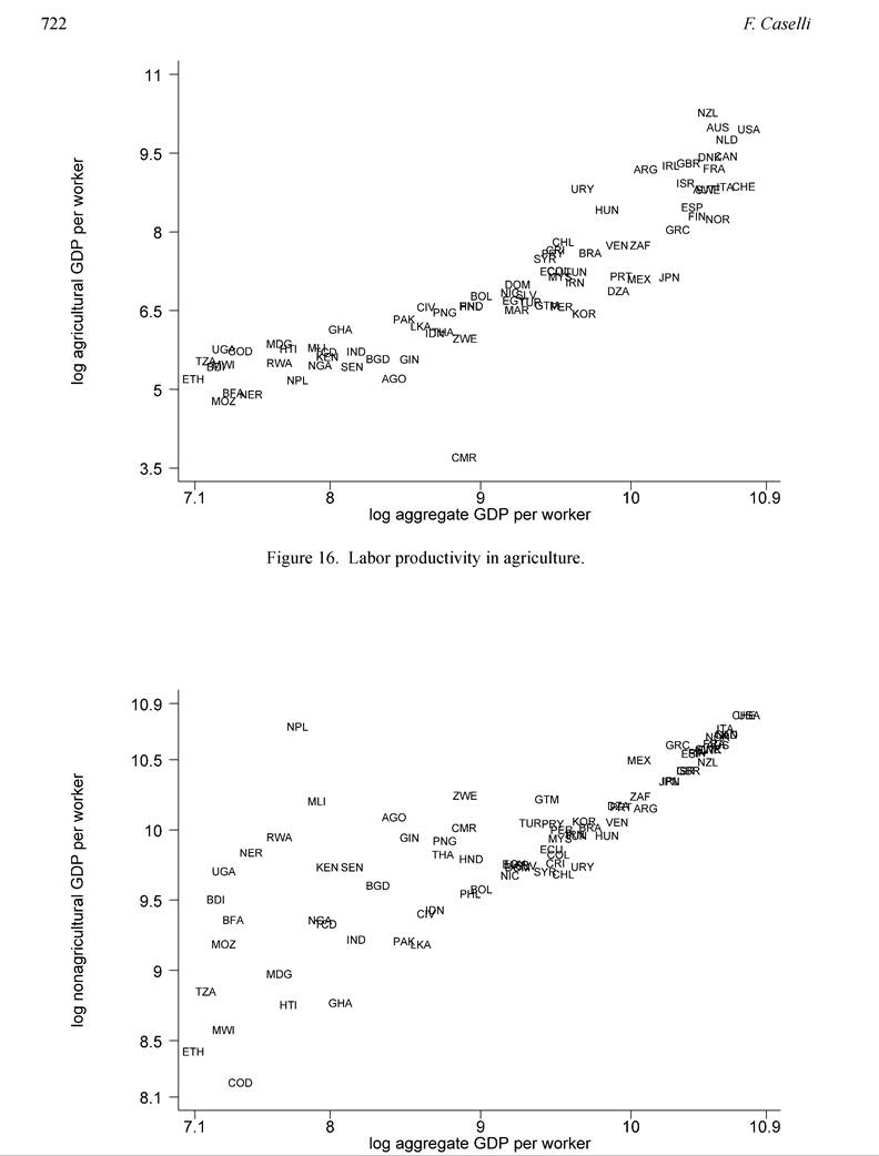
Figure 17. Labor productivity outside of agriculture.

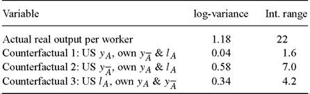
Table 4

Counterfactual World income distributions

Recalling now from Figure 15 that the third component of Equation (12), the em­ployment share l_A, ranges from almost 0 percent in the richest countries to almost 100 percent in the poorest, we conclude that poor countries have most of their labor force in the sector where they are particularly unproductive.^58,59

We can summarize this first overview of the sectorial data by saying that there are three proximate reasons for poor countries’ poverty: their much lower labor productivity in agriculture; their somewhat lower labor productivity outside agriculture; and their larger share of employment in the sector that - on average - is less productive.

To quantify these effects Table 4 presents income-dispersion statistics (log-variance and inter-percentile range) in the data (first row), and under alternative counterfactual assumptions on industry-level productivity and labor shares.

⁵⁸ Attempts at explaining this apparent deviation from comparative advantage abound. It may be that the non- agricultural sector has greater skill requirements, so that low human-capital economies are constrained in the supply of non-agricultural workers [Caselli and Coleman (2001b)]; or it could be that investment distortions push producers into the home (agricultural) sector [Gollin, Parente and Rogerson (2000)]; or it could be that economies are subject to a “subsistence constraint”, such that resources cannot start moving out of agriculture until agriculture is sufficiently productive to generate a surplus that will feed the industrial class [Gollin, Par­ente and Rogerson (2001); Restuccia, Yang and Zhu (2003)]; or it could be that some countries are “trapped” in agriculture by a coordination failure [long tradition; most recently Graham and Temple (2001)].

⁵⁹ Given the huge employment shares of agriculture in Figure 15 one would guess that in most developing countries agriculture would account for an equally vast share of GDP. In fact, the agricultural share of GDP is always below 40 percent. This is a consequence of the disproportionately low productivity of agriculture in low-income countries. Also note that the PPP agricultural share in GDP is both much less variable across countries, and - for most countries - lower than the domestic-currency agricultural share in GDP. This is because - perhaps contrary to common wisdom - the relative price of agricultural goods is higher in poor countries than in the US.

⁶⁰ A similar calculation is reported by Restuccia, Yang and Zhu (2003). Calculations in this spirit can also be found in Caselli and Coleman (2001b) (for US regions), and Gollin, Parente and Rogerson (2001).

The results are stunning. The figures in the second row imply that if poor countries achieved the same level of agricultural labor productivity as the US, world income in­equality would virtually disappear! This is of course a reflection of the convergence of US agricultural incomes to US non-agricultural incomes [documented in Caselli and Coleman (2001b)], as well as the huge agricultural share of employment in many of the poorest countries. However, the other two counterfactual experiments also gener­ate large declines in dispersion. Because agriculture is generally much less productive than non-agriculture, reducing the agricultural employment share to US levels would reduce income inequality by an enormous two thirds (third row). And cross-country non-agricultural productivity differences, while much less than agricultural ones, are still sufficiently large that income inequality would fall by about one half if poor coun­tries were as productive outside of agriculture as the US (second row).⁶¹

6.3. Sectorial composition and development accounting

The previous subsection establishes that there are very large within industry cross­country differences in output per worker. Indeed, the agricultural GDP differences are substantially larger than the aggregate GDP ones. Furthermore, these cross-country differences in industry GDPs are seen to potentially “account” for a large fraction of the cross-country dispersion in aggregate income. We can now return to the original question: are these large differences in agricultural GDP attributable to the amounts of observable inputs employed in agriculture by the various countries, or are they the result of industry-level cross-country TFP differences? This is of course “the” development­accounting question.

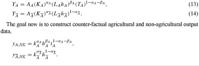
To try to answer this question, we need assumptions on the industry production func­tions, as well as ways of measuring industry-level inputs. I will assume that each of the two sectors produces according to a Cobb-Douglas technology. In agriculture, the factors of production are capital, labor, and land (T). In non-agriculture, they are capital and labor:

^[1] Of course, this discussion abstracts from the changes in world-wide agricultural relative prices that such changes would bring about.

These counter-factual data answer the question: what would the world distribution of agricultural (non-agricultural) output per worker look like if all countries had the same agricultural (non-agricultural) total factor productivity?

Assume that the rates of return on capital must be equalized across sectors - a plau­sible arbitrage condition. This is easily seen to imply

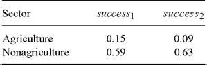
Table 5

Success within sectors

and

Since y_A and y^ are known, we can back out reference values for P_aA_a and P_aA^ and compute the counter-factual in (16). The result of this exercise, which is also the main result of this section, is 0.34 for success₁, and 0.32 for success₂. In words, once again, this means that, if all countries had the same industry-level TFPs as the US, but their observed allocation of measurable factors to agriculture and non-agriculture, the world distribution of income would be about one third as unequal as it actually is. Given that - for this sub-sample - the corresponding success measures are 0.45 and 0.39 when the sectorial composition of GDP is not taken into account, I conclude that taking account of differences in sectorial composition actually decreases the share of cross-country income inequality that we can explain with a country’s factor endowments.

This result should have been expected, by now. In the previous subsection we have seen that the dispersion in agricultural incomes per worker is a critical “source” of dispersion in per-capita income. Table 5 shows, however, that almost all of the variation in agricultural income comes from differences in agricultural TFP. It is not surprising, therefore, that we find that - even allowing for differences in output composition - factor endowments still do not work as the main cause of GDP differences.

One possible way to enhance the quantitative role of sectorial considerations is ex­plored in a highly innovative paper by Graham and Temple (2001). Instead of assuming, as here, that both agriculture and non-agriculture have constant returns to scale, they follow a long tradition in development economics in hypothesizing that the former is characterized by decreasing returns and the latter by increasing returns. As is well known these assumptions tend to generate multiple equilibria, and it is therefore possi­ble to try to explain large cross-country income differences with the argument that poor countries are in “low”, i.e. high agriculture, i.e. low returns, equilibria; while rich coun­tries are in industrialized equilibria and therefore benefit from the increasing returns. The difficulty here is to figure out in the data which countries are in the bad and which ones are in the good equilibrium. The contribution of Graham and Temple is to show a very ingenious way of solving this problem. They find that multiple equilibria explain a relatively large fraction of per capita income differences. The lingering question is whether the significant departures from constant returns to scale required for their result are plausible.⁶⁴