Quality of physical capital
4.1. Composition
Recent research by Eaton and Kortum (2001) has shown that most of the world’s capital is produced in a small number of R&D-intensive countries, while the rest of the world generally imports its equipment.
This suggests that, for most countries, (widely available data on) imports of capital of a certain type are an adequate proxy for overall investment in that type of equipment. Caselli and Wilson (2004) exploit this observation to investigate cross-country differences in the composition of the capital stock.[407]Their results - a partial summary of which is shown in Table 3 - are startling: different types of equipment constitute widely varying fractions of the overall capital stock across countries. For each of the nine equipment categories Caselli and Wilson work with, the share in total investment in 1995 has minima in the low single digits, and maxima
Table 3
The composition of the capital stock
| Fabricated metal products | Nonelectrical machinery | Office computing accounting | Electrical equipment | Comm. equipment | Motorvehicles | Other transp. | Aircraft | Prof. goods | |
| Mean | 0.08 | 0.21 | 0.06 | 0.14 | 0.11 | 0.24 | 0.03 | 0.05 | 0.07 |
| STD | 0.06 | 0.08 | 0.05 | 0.07 | 0.05 | 0.10 | 0.04 | 0.09 | 0.03 |
| Min | 0.01 | 0.03 | 0.01 | 0.01 | 0.01 | 0.01 | 0.00 | 0.00 | 0.01 |
| Max | 0.55 | 0.48 | 0.41 | 0.59 | 0.37 | 0.55 | 0.34 | 0.88 | 0.23 |
| CorrY | -0.25 | -0.14 | 0.53 | 0.27 | 0.20 | -0.32 | -0.41 | 0.14 | 0.33 |
| R&D | 202 | 887 | 1170 | 848 | 2280 | 1810 | 57 | 1880 | 801 |
that vary between 20 percent and 80 percent! The standard deviations of investment shares are always large relative to the cross-country means.
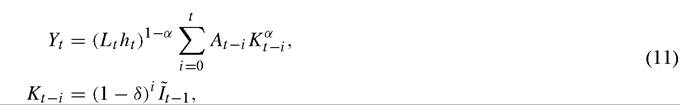
Furthermore, this enormous heterogeneity is systematically related to per capita income, as the correlations with income of the various investment shares are large in absolute values.To begin to see why this vast heterogeneity in the composition of equipment may matter for development-accounting, Table 3 also reports global, cumulated R&D expenditures in the various equipment categories.[408] The wide variation in R&D spending across types reinforces the impression of equipment heterogeneity across countries: since equipment shares vary so much, so does the embodied-technology content of the aggregate capital stock. If the R&D content of equipment determines its quality, i.e. its productivity per dollar of market value, one begins to suspect that the quality of capital - and not only its quantity - may vary across countries.
Furthermore, these differences are systematic, since richer countries appear to employ high R&D capital much more than poor countries. A simple way to see this is to look at Figure 14, from Wilson (2004). For equipment types with a high R&D content the share in overall investment is positively correlated with output per worker, while the opposite is true for low-tech equipment types. Could it be that rich countries use higher quality equipment, and that this higher quality accounts for some of the residual TFP variance?
To see how this may work it is useful to write down a very simple model. Imagine that final output Y is produced combining various intermediate inputs, χp, according to the CES production function[409]
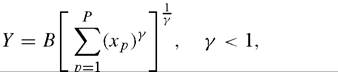
Figure 2: R&D flow intensity (%) vs. Corr(Y∕L, import share) 1995, 118 countries
0.6
Office and Computer Eq.
0.53
0.4

0.2
lBectrical Eq.
0.27
• Professional Goods
0.33
0-----
0.(00
• Communications Eq.
0.20
Aircraft
0.14
0.020 0.040 0.060 0.080 0.100 0.120 0.140 0.160 0.180
o.; 00
-0.2
-0.4
_ Non-electrical Eq.
-0.14
• Fabricated Metal
• Motor Vehicles -0.32
• Other Trans. Eq. -0.41
-0.25
-0.6
R&D Intensity
Figure 14. Capital composition and income.
where B is a disembodied total factor productivity term. Intermediate-good p is produced combining equipment and labor:
Xp = Ap(hpLp)l~α(Kp)α, 0 < α < 1, (9)
where Kp measures the quantity of equipment (in current dollars) used to produce intermediate-input p, hpLp is human-capital augmented labor in sector p, and Ap is the productivity of sector p.
The key assumption is that capital is heterogeneous: there are P distinct types of capital, and each type is product specific, in the sense that intermediate p can only be produced with capital of type p. In other words, an intermediate is identified by the type of equipment that is used in its production.[410] The assumption that γ < 1 implies that - in producing aggregate output - all these activities are imperfect substitutes.
The productivity term Ap is product specific. Product variation in A allows for the possibility that one dollar spent on equipment of type p may deliver different amounts of efficiency units if instead spent on type p'. For example, the embodied-technology content of good p may be greater because the industry producing equipment of type p is more R&D intensive.[411]
A number of simplifying assumptions allow one to write a simple formula that brings the idea of the “quality of capital” in sharp relief. In keeping with the representativeagent spirit of the rest of the chapter say, then, that human capital per worker is constant across sector, i.e.
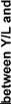
hp = h, and that labor is free to flow across sectors so that the marginal product of labor is the same for all equipment types. Then one can show that the output equation can be rewritten as[412]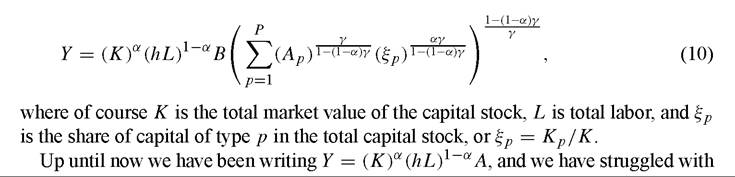
the fact that A seems to play an enormously important role in determining output differences. The last equation neatly shows the relationship between A and the composition of the capital stock: if different types of capital have different productivities, then the observed wild variation in equipment shares ξ implies that the quality of capital - over and above its quantity K - can vary across countries and can account for a portion of the unexplained variation.
Caselli and Wilson (2004) propose a regression-based approach to make inferences on the various Ap s. Unfortunately, even with knowledge of the Ap s it is virtually impossible to bound the amount of income variance that the ξp s can explain. This is because the last term of Equation (10) is exceedingly sensitive to the value of γ, and there seem at the moment to exist no reliable approach to the calibration of this elasticity. If γ is sufficiently low, i.e. capital types are sufficiently poor substitutes for one another, the quality of capital accounts for all of the unexplained component of income differences. However, whether such values are reasonable or not our current state of knowledge cannot say. I conclude therefore that further research on the composition of capital is an important priority for development accounting.
5.2. Vintage effects
Solow’s (1959) paper on vintage capital formalized the idea that technological progress is embodied in capital goods. Rodriguez-Clare (1996), Jovanovic and Rob (1997), Parente (2000), Mateos-Planas (2000) have noted that this could potentially enhance the explanatory power of cross-country differences in investment rates.
The idea, of course, is that low investment rates will be associated with lower adoption of new technology. Indeed, some of these authors have argued that versions of the capital-embodied model greatly outperform the homogeneous-capital model in accounting for cross-country income differences.Formally, the vintage-capital model could be described by the formulas:
where It-1 is investment at time t — 1 in terms of the consumption good. Consistent with Solow’s idea, this model has the property that capital installed by sacrificing one unit of consumption at date s yields As(1 — δ)t-s efficiency units of capital at time t, while capital installed by sacrificing one unit of consumption at time t yields At efficiency units. If As < At we have that the earlier sacrifice in consumption contributes less to output today not only because of physical depreciation, but also because of the older vintage. To appreciate the potential consequences of this note that the same comparison in a homogeneous-capital (i.e. disembodied technical change) model would be between At(1 — δ)t-s and At, i.e. differences in efficiency units obtained with the same sacrifice of consumption would only be due to physical depreciation.
As explained by Greenwood, Hercowitz and Krusell (1997), under certain conditions the formulation above is equivalent to
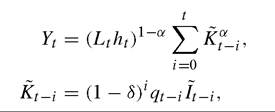
which has the following interpretation. Instead of one unit of consumption producing equal amounts of capital of increasing quality at different dates, one unit of consumption produces increasing amounts of capital of the same quality. Because the aggregate implications of growth in A are isomorphic to those of growth in q,the two formulations can be equivalent representations of the idea of embodied technological progress.
The second version of the model suggests, however, that - at least in principle - the estimates of the physical capital stocks we have been using until now do actually already reflect embodied technical change. This is because the real investment series we construct from PWT61 is a series for real investment in terms of the investment good, and not in terms of the consumption good. In other words, the PWT61 investment data
that we use are data on Is = qsIs, and not on Is. Therefore, vintage effects - or at least those vintage effects that show up in a reduced relative price of investment goods - should already be accounted for.
As a very rough check on this argument, I have run a cross-country OLS regression of output per quality-adjusted worker on a distributed-lag function of depreciated investments (in units of the investment good). I.e. the left hand side variable was Yt∕(Ltht)1-α, and the right hand side variables were It, (1 - δ)It-1, (1 - δ)2It-2,.... I experimented with 5, 10, and 20 lags of investment. The homogeneous-capital hypothesis - or, much more accurately, the hypothesis that all vintage effects are adequately captured by investment-good prices in PWT61 - is equivalent to all the coefficients taking the same value, irrespective of the vintage. The “vintage effects” hypothesis would predict that coefficients on recent lags of investment would be systematically larger than those on older lags. The result was somewhat inconclusive, in that both hypotheses were rejected: all coefficients were not statistically the same, but neither they fell monotonically with the lag of investment. A possible explanation is that the price deflators in PWT work well enough to remove systematic vintage effects, but the remaining i.i.d. measurement error occasionally makes some vintages look more productive than others. Inany case there is little indication that vintage-based models will significantly improve on the benchmark.
5.3. Further problems with K
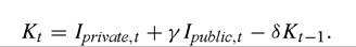
The investment series I have used to estimate the capital stock is an aggregate of private and public investment expenditures. As Pritchett (2000) very convincingly argues, however, elementary logic and vast anecdotal experience suggest that many governments’ investment efforts are much less productive than private ones. There is an infinite supply of examples where government investments have not produced anything tangible (non-existent highways, industrial complexes that have never been completed, etc.). Furthermore, even when public investments do materialize, the resulting structures and machinery may be run less efficiently than under private management.[413]
As for Pritchett’s (2003) criticism of schooling-based measures of human capital based on private returns, his (2000) criticism of what he derogatorily but accurately calls CUDIE (cumulated depreciated investment expenditure) may help shedding light on the puzzles we are concerned with, both because governments tend to account for a larger share of production, employment, and capital ownership in poorer countries, and because less-accountable poor-country governments are likely to be disproportionately less efficient (relative to the private sector) than rich country ones. Hence, there are good reasons to expect the government to play an especially detrimental role in the productivity of investment in poor countries. This implies that the “effective” variance of K is larger than in the baseline model.[414]
As I suggested in the previous section for the analogous problem with human capital, a first pass at investigating this issue would be to try to separate out public from private investment, and apply different weights in the perpetual-inventory calculation, which would become
One could then try to re-do development accounting with this modified capital measure (possibly for various values of γ). Unfortunately, I have not been able to identify reliable and updated PPP breakdowns of the investment series into private and public capital.[415]
Perhaps a cleaner exercise, but also even more ambitious, would be to try to completely net out the government from the development accounting exercise. I.e. subtract the government’s share from aggregate output, capital ownership, and employment, and perform the development-accounting exercise on the residual (private) inputs and output. This confronts the same data limitations as the exercise described in the previous paragraph, and the additional problem of coming up with a reliable PPP government share of GDP[416]
6.
More on the topic Quality of physical capital:
- Quality of Bedding
- Capital adequacy management
- Empirical studies of the effects of social capital
- THE ECONOMIC VALUE OF DATA IN BIG DATA
- Productivity and labour skills
- Growth and development
- THE IMPACT OF INTERNET ARCHITECTURE ON THE ECONOMIC ENVIRONMENT FOR APPLICATION INNOVATION
- The economics of the environment
- 12 The Dragon Goes to Sea