The economics of the environment

In recent years, there has been considerable interest in the impact of economic decisions on the environment.

In this chapter we start by reviewing the position of the environment in models of national income determination.

I The role of the environment

The familiar circular flow analysis represents the flow of income (and output) between domestic firms and households. Withdrawals (leakages) from the circular flow are identified as savings, imports and taxes, and injections into the circular flow as investment, exports and government expenditure. When withdrawals exactly match injections, then the circular flow is regarded as being in ‘equilibrium’, with no further tendency to rise or fall in value.

All this should be familiar from any introductory course in macroeconomics. This circular flow analysis is often considered to be ‘open’ since it incorpor­ates external flows of income (and output) between domestic and overseas residents via exports and imports. However, many economists would still regard this system as ‘closed’ in one vital respect, namely that it takes no account of the constraints imposed upon the economic system by environmental factors.

Figure 10.1 provides a simplified model in which linkages between the conventional economy (circular flow system) and the environment are now intro­duced. The natural environment is seen as being involved with the economy in at least three specific ways.

1 Amenity Services (A). The natural environment provides consumer services to domestic house­holds in the form of living and recreational space, natural beauty and so on. We call these ‘Amenity Services’.

2 Natural Resources (R). The natural environment is also the source of various inputs into the produc­tion process such as mineral deposits, forests, water resources, animal populations and so on. These natural resources are, in turn, the basis of both the renewable and non-renewable energy supplies used in production.

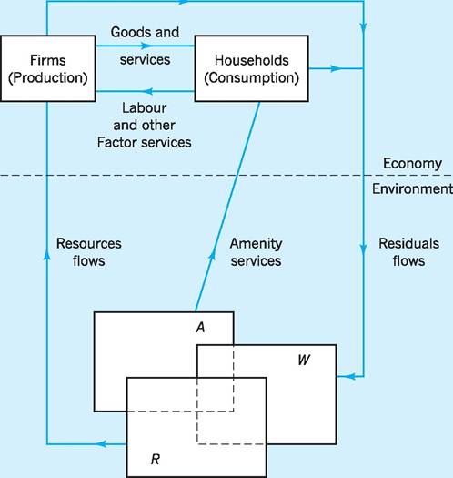
Fig. 10.1 Economy/environment linkages.

3 Waste Products (W). Both production and con­sumption are activities which generate waste prod­ucts or residuals. For example, many productive activities generate harmful by-products which are discharged into the atmosphere or watercourses. Similarly, sewage, litter and other waste products result from many consumption activities. The key point here is that the natural environment is the ultimate dumping place or ‘sink’ for all these waste products or residuals.

We have now identified three economic functions of the environment: namely, it functions as a direct source of consumer utility (A), as a resource supplier (R) and as a waste receptor and assimilator (W). Moreover, these functions interact with other parts of the economic system and also with each other. This latter point is the reason for showing the three boxes A, R and W as overlapping each other in Fig. 10.1. For example, a waterway may provide amenity ser­vices (A) to anglers and sailors, as well as aesthetic beauty to onlookers.

By bringing the environment into our modelling of the economy, we are essentially challenging the tradi­tional view that the environment and the economy can be treated as separate entities. Everything that happens in the economy has a potential environ­mental impact. For example, excessive price support for agricultural products under the Common Agri­cultural Policy (CAP - see Chapter 29) will encourage over-production of agricultural produce. Land which might otherwise be left in its natural state may then be brought into agricultural use, and increased yields may be sought by additional applications of fertilizers and pesticides. Hedgerows may be cut back to pro­vide larger and more economical units of cultivation, and so on. In other words, most types of economic policy intervention will impact upon the environment directly or indirectly. Equally, policies which seek to influence the environment will themselves impact upon the economic system. As we shall see, attempts to reduce CO₂ (carbon dioxide) emissions may influ­ence the relative attractiveness of different types of energy, causing consumers to switch between coal, gas, electricity, nuclear power and other energy forms.

Sustainable economic welfare

Rather more sophisticated attempts to capture envir­onmental costs within a national accounting frame­work have been made in recent years. For example, an Index of Sustainable Economic Welfare (ISEW) has been calculated for the US and UK. Essentially, any increase in the GNP figure is adjusted to reflect the following impacts which are often associated with rising GNP:

■ monies spent correcting environmental damage (i.e. ‘defensive’ expenditures);

■ decline in the stock of natural resources (i.e. environmental depreciation);

■ pollution damage (i.e. monetary value of any environmental damage not corrected).

By failing to take these environmental impacts into account, the conventional GNP figure arguably does not give an accurate indication of sustainable eco­nomic welfare, i.e. the flow of goods and services that an economy can generate without reducing its future production capacity. Suppose we consider the expenditure method of calculating GNP. It could be argued that some of the growth in GNP is due to expenditures undertaken to mitigate (offset) the impact of environmental damage. For example, some double­glazing may be undertaken to reduce noise levels from increased traffic flow, and does not therefore reflect an increase in economic wellbeing, merely an attempt to retain the status quo. Such ‘defensive expenditures’ should be subtracted from the GNP figure (item 1 above). So too should be expenditures associated with a decline in the stock of natural resources. For example, the monetary value of miner­als extracted from rock is included in GNP, but noth­ing is subtracted to reflect the loss of unique mineral deposits. ‘Environmental depreciation’ of this kind should arguably be subtracted from the conventional GNP figure (item 2 above).

We are then left with an Index of Sustainable Eco­nomic Welfare (ISEW) which subtracts rather more from GNP than the usual depreciation of physical capital.

ISEW = GNP minus depreciation of physical capital minus defensive expenditures minus depreciation of environmental capital

minus monetary value of residual pollution

The effect of such adjustments is quite startling. The UK GNP per capita (unadjusted) has grown by around 2.0% in real terms as an annual average in the UK since 1950. However, the adjustment out­lined above for each year over the period gives an ISEW per head for the UK which corresponds to a mere 0.5% average annual growth in real ISEW over the period. Such ‘environmental accounting’ is sug­gesting an entirely different perspective on recorded changes in national economic welfare.

I Valuing the environment

A number of approaches may be used in seeking to place a ‘value’ on environmental changes, whether ‘favourable’ (benefits) or ‘unfavourable’ (costs). Some­times the market mechanism may help in terms of monetary valuations by yielding prices for products derived from environmental assets. However, these market prices may be distorted by various types of ‘failure’ in the market mechanism (e.g. monopolies or externalities), so that some adjustment may be needed to these prices. For example ‘shadow prices’ may be used, i.e. market prices which are adjusted in order to reflect the valuation to society of a particular activity.

On other occasions there may be no market prices to adjust, in which case we may need to use ques­tionnaires to derive hypothetical valuations of ‘willingness to pay’ for an environmental amenity or ‘willingness to accept’ compensation for an envir­onmental loss.

The issue of time is particularly important for monetary valuation of environmental impacts which may take many years to materialize. It is therefore important to pay close attention to the process of calculating the present value of a stream of future revenues or costs, using the technique of discounting (see Chapter 17, p. 341).

We return to these valuation techniques below, but first it will be useful to consider why valuing environmental costs and benefits is so important to policy-makers.

Finding the socially optimum output

Figure 10.2 presents a simplified model in which the marginal pollution costs (MPC) attributable to production are seen as rising with output beyond a certain output level, Q_A. Up to Q_A the amount of pollution generated within the economy is assumed to be assimilated by the environment with zero pollu­tion costs. In this model we assume that pollution is a ‘negative externality’, in that firms which pollute are imposing costs on society that are not paid for by those firms.

At the same time the marginal net private benefit (MNPB) of each unit of output is assumed to decline as the level of economic activity rises. MNPB is the addition to private benefit received by firms from

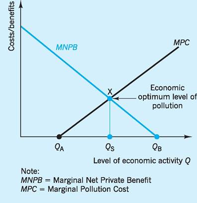
Fig. 10.2 Finding an optimum level of pollution.

selling the last unit of output minus the addition to private costs incurred by producing that last unit of output.

If the pollution externality was not taken into account, then firms would produce up to output QB at which MNPB = 0. Only here would total net pri­vate benefit (i.e. total profit) be a maximum. However, the socially optimum level of output is Q_s, where MNPB = MPC. Each unit of output beyond Q_s adds more in pollution costs to society than it does to net private benefit, and is therefore socially inefficient to produce. Equally it would be socially inefficient to forsake producing any units up to Q_s, since each of these units adds more to net private benefit than to pollution costs for society.

Note that in this analysis the social optimum does not imply zero pollution. Rather it suggests that the benefits to society are greatest at output Q_s, with pol­lution costs being positive at Q_sX. We return to this idea of seeking ‘acceptable’ levels of pollution below.

The valuation issue

A key element in finding any socially efficient solution to the negative environmental effects of increased production clearly involves placing a monetary value on the marginal private and social costs (or benefits) of production. In terms of Fig. 10.2 we need some monetary valuation which will permit us to estimate both the MNPB and the MPC curves.

Using ‘shadow prices'

Where market prices exist, it is at least feasible to obtain monetary valuations of future net revenues from an environmental asset. However, where one or more market failures occur, these prices may be deemed ‘inappropriate’ and in need of adjustment to reflect more accurately the true benefits and costs to society. Such adjustments give rise to ‘shadow prices’, i.e. prices which do not actually exist in the market­place but which are assumed to exist for purposes of valuation.

Demand curve methods

‘Expressed preference’ and ‘revealed preference’ methods are widely used here.

Expressed preference methods

Where no market price exists, individuals are often asked, using surveys or questionnaires, to express how much they would be willing to pay for some speci­fied environmental improvement, such as improved water quality or the preservation of a threatened local amenity. In other words, an ‘expressed preference’ approach is taken to valuation. An example of the use of this approach was used in Ukunda, Kenya, where residents were faced with a choice between three sources of water - door-to-door vendors, kiosks and wells - each requiring residents to pay different costs in money and time. Water from door-to-door vendors cost the most but required the least collection time. A study found that the villagers were willing to pay a substantial share of their incomes - about 8% - in exchange for this greater convenience and for time saved. Such valuations can be helpful in seeking to make the case for extending reliable public water supply even to poorer communities. Questionnaires and surveys of willingness to pay have been widely used in the UK to evaluate the recreational benefits of environmental amenities. They can help capture ‘use value’ (see p. 193) where market prices are inappropriate or do not even exist, as well as ‘option’ and ‘existence’ values.

These ‘expressed preference’ methods are some­times referred to as ‘contingent valuation’ methods, since the user’s ‘willingness to pay’ (WTP) is often sought for different situations ‘contingent upon’ some improvement in the (environmental) quality of provi­sion. The same approach may involve asking indi­viduals how much they are ‘willing to accept’ (WTA) to avoid some specific environmental degradation.

Revealed preference methods

This approach seeks to avoid relying on the use of questionnaires or surveys to gain an impression of the hypothetical valuations placed by consumers on various environmental costs and benefits. Instead it seeks to use direct observation of the consumers’ actual responses to various substitute or complemen­tary goods and services to gain an estimate of value in a particular environmental situation. The focus here is on the ‘revealed preferences’ of the consumers as expressed in the marketplace, even if this expression is indirect in that it involves surrogate goods and services rather than the environmental amenity itself.

1 Travel Cost Method (TCM). Where no price is charged for entry to recreational sites, economists have searched for private market goods or services whose consumption is complementary to the con­sumption of the recreational good in question. One such private complementary good is the travel costs incurred by individuals to gain access to recreational sites. The ‘price’ paid to visit any site is uniquely determined for each visitor by calculating the travel costs from his or her location of origin. By observing people’s willingness to pay for the private complementary good it is then possible to infer a price for the non-price environmental amenity.

In Fig. 10.3, the demand curve D_visits shows the overall trend relationship between travel costs and visit rates for all the visitors interviewed. Using this information we can estimate the average visitor’s (V₁) total recreational value (V₁ ? P₁) for the site. Multiplying this by the total number of visitors per annum allows us to estimate the total annual recreational value of the site.

2 Hedonic Price Method (HPM). A further tech­nique often used in deriving valuations where no prices exist is the so-called ‘hedonic price’ method. This estimates the extent to which people are, for example, willing to pay a house price premium for the benefit of living within easy access of an environmental amenity. It could equally be used to estimate the house price discount resulting from living within easy access of a source of environ­mental concern.

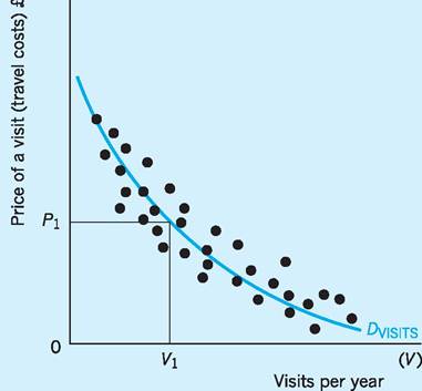
Fig. 10.3 The relationship between the number of visits to a site and the price of the visit.

House and other property prices are clearly deter­mined by a number of independent variables. some of these will involve variables related to the following.

■ Characteristics of the property: number of rooms, whether detached, semi-detached or terraced, garage facilities available, etc.

■ Characteristics of the location: number (and repu­tation) of schools, availability of shopping and recreational facilities, transport infrastructure, etc.

■ Characteristics of the environment: proximity to favourable or unfavourable environmental factors.

Statistical techniques (such as multiple regression analysis) can be used to estimate the influence of these possible ‘explanatory’ (independent) variables on house and property prices. For example, a ‘classic’ statistical study of the impact of traffic noise in Washington, DC, established an inverse relationship between house prices and the environmental factor ‘noise pollution’ with each extra decibel of noise found to be statistically correlated with a 0.88% fall in average house prices.

Non-demand curve valuations

Essentially both the expressed preference and revealed preference methods are making use of demand curve analysis in placing monetary values on aspects of environmental quality. However, a number of valuation methods may be used which depart from this approach.

Replacement cost method

The focus here is on the cost of replacing or restoring a damaged asset. This cost estimate is then used as a measure of the ‘benefit’ from such replacement or restoration. For example, if it costs £1m to restore the facade of buildings damaged by air pollution, then this £1m cost is used as an estimate of the benefit of environmental improvement.

Preventative expenditure method

The focus here is on using the costs incurred in an attempt to prevent some potential environmental damage as a measure of ‘benefit’. For example, the expenditure incurred by residents on double-glazing to avoid ‘noise pollution’ from a new trunk road might be used as a proxy variable of the value placed by residents on noise abatement.

Delphi method

The focus here is on valuations derived from consult­ing a group of recognized experts. Each member of the group responds independently to questions as to the valuations that might be placed on various (envir­onmental) contingencies in their area of expertise. The initial responses of the group are then summar­ized in graphical or tabular form, with each member given the opportunity to re-evaluate their individual responses. The idea here is that through successive rounds of re-evaluation, a consensus valuation of the expert group may eventually emerge.

Cost-benefit analysis (CBA)

Under cost-benefit analysis, the techniques already discussed and others are used to assign monetary values to the gains and losses to different individuals and groups, often weighted according to some per­ception of the contribution of these individuals or groups to social utility (social welfare). It is for this reason that this approach is sometimes referred to as ‘social’ cost-benefit analysis. Some of the ‘market failures’ previously identified are taken into account, with some existing market prices adjusted (e.g. via weighting) and values attributed to some situations where no market prices currently exist. If the pro­posed reallocation of resources via new investment in some (environmental) project is evaluated as creating benefits that are greater, in present value terms, to those who gain than the costs imposed on those who lose, then the project is potentially viable from soci­ety’s perspective. In other words, if the net present value to society of a project is positive, then the pro­ject is at least worthy of consideration. Whether or not it will be undertaken may depend upon what restrictions, if any, apply to the level of resources (finance) available. If such resources are limited and must be rationed, then of course only those projects with the highest (positive) net present values to soci­ety may be selected.

Total economic value

In recent years there has been considerable discussion as to how to find the ‘total economic value’ (TEV) of an environmental asset. The following identity has been suggested:

Total economic value ? use value + option value

+ existence value

The idea here is that ‘use value’ reflects the prac­tical uses to which an environmental asset is currently being put. For example, the tropical rainforests are used to provide arable land for crop cultivation or to rear cattle in various ranching activities. The forests are also a source of various products, such as timber, rubber, medicines, nuts, etc. In addition, the forests act as the ‘lungs’ of the world, absorbing stores of carbon dioxide and releasing oxygen, as well as help­ing to prevent soil erosion and playing an important part in flood control.

There are clear difficulties in placing reliable monet­ary estimates on all these aspects of the ‘use value’ of the rainforest. However, it is even more difficult to estimate ‘option value’, which refers to the value we place on the asset now as regards functions which might be exploited some time in the future. For example, how much are we willing to pay to preserve the rain­forest in case it becomes a still more important source of herbal and other medicines? This is a type of insur­ance value, seeking to measure the willingness to pay for an environmental asset now, given some probability function of the individual (or group) wishing to use that asset in various ways in the future.

Finally, ‘existence value’ refers to the value we place on an environmental asset as it is today, inde­pendently of any current or future use we might make of that asset. This is an attempt to measure our willingness to pay for an environmental asset simply because we wish it to continue to exist in its present form. Many people subscribe to charities to preserve the rainforests, other natural habitats or wildlife even though they may never themselves see those habitats or species. Existence value may involve inter-generational motives, such as wishing to give one’s children or grandchildren the opportunity to observe certain species or ecosystems.

Although much remains to be done in estimating TEV, a number of empirical studies have been under­taken. For instance, the Flood Hazard Research Centre in the UK estimated that in 1987/88 people were willing to pay £14 to £18 per annum in taxes in order that recreational beaches (use value) be protected from erosion (Turner 1991). The researchers also surveyed a sample of people who did not use beaches for recreational use. They estimated that these people were willing to pay £21 to £25 per annum in taxes in order to preserve these same beaches (existence value).

Overall, many estimates are finding that the ‘option’ and ‘existence’ values of environmental assets often far exceed their ‘use’ value. For example, existence values for the Grand Canyon were found to outweigh use values by the startling ratio of 60 to 1 (Pearce 1991a). In similar vein, non-users of Prince William Sound, Alaska, devastated by the Exxon Valdez oil spill in 1989, placed an extremely high value on its existence value (O’Doherty 1994). The amounts non-users were estimated (via interviews) as willing to pay to avoid the damage actually incurred came to $2.8bn, i.e. $31 per US household. This approach, whereby interviewees are asked about the value of a resource ‘contingent’ on its not being damaged, is often termed ‘contingent valuation’.

We now turn to the important policy issue of how we can provide market incentives or regulations which will result in a socially optimum level of environ­mental damage (output Q_s in Fig. 10.2), rather than the higher levels of environmental damage which would result from an unfettered free market in which externalities were ignored (output Q_b in Fig. 10.2).

Market-based and non-market- based incentives

In free-market or mixed economies the market is often seen as an efficient means of allocating scarce resources. Here we look at ways in which the market could be used to provide incentives to either firms or consumers in order to bring about a more socially optimum use of environmental assets.

Market-based incentives

Environmental taxes

An environmental tax is a tax on a product or service which is detrimental to the environment, or a tax on a factor input used to produce that product or ser­vice. An environmental tax will increase the private costs of producing goods or services which impose negative ‘externalities’ on society.

In Fig. 10.4 we have a situation similar to that in Fig. 10.3 with Q_s as the socially optimum output. The marginal pollution costs (MPC) curve is more usually referred to as the marginal external cost (MEC) curve, as the firm is imposing these pollution costs but not, initially, paying for the damage done. In terms of Fig. 10.4, if a lump-sum tax of t is now imposed on the polluter, it has the effect of shifting the MNPB curve downwards and to the left, thus giv­ing MNPB - t. Remember that MNPB is the marginal profit (see p. 190) on each extra unit produced which is now reduced by the tax t levied on each unit. The polluter would now maximize total net private bene­fits (i.e. total profit) at a level of activity equal to Q_s.

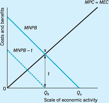
Fig. 10.4 I mposing a lump-sum environmental tax t on output.

If the firm produced an amount greater than Q_s then it would pay more in costs and tax on the extra units sold than it would receive in revenue (profit would fall). If the firm produced an amount less than Q_s then it would pay less in costs and tax on the extra units sold than it would receive in revenue (profit would rise). Only at output Q_s is total net private benefit (total profit) a maximum, i.e. where MNPB - t = 0. The tax would be equal to MEC at the optimum level of pollution.

Using environmental taxes in this way is often said to be a policy of ‘internalizing’ the externality. In other words, the firm itself now has the incentive to take the externality into account in its own decision­making. There are, however, problems with using an environmental tax, not least in determining the tax rate (t) which will make MNPB - t = 0.

A move towards environmental taxes is in line with the ‘polluter pays’ principle adopted by the OECD in 1972. This principle states that ‘the polluter should bear the cost of measures to reduce pollution decided upon by public authorities to ensure that the environment is in an “acceptable state”’. The idea behind adopting this principle across member states was to avoid the distortions in comparative advan­tages and trade flows which could arise if countries tackled environmental problems in widely different ways. Slightly less than 2% of UK total tax revenue is currently yielded by explicitly environmental taxes, although if general taxes on energy are also included in a looser definition of ‘environmentally related’ taxes, then this figure rises to some 8.5% of UK total tax revenue.

An environmental subsidy can be thought of as a negative environmental tax. If in Fig. 10.4, the opti­mum social output was to the right of Q_p, then the policy prescription might be a subsidy rather than a tax. A subsidy would shift the MNPB upwards by the amount of the subsidy (v), giving MNPB + v, and total net private benefit (profit) would be maximized at an output to the right of Q_p. In an attempt to encourage farmers to reforest agricultural land, China is paying farmers $450 a year per reforested hectare in the area around the Yangzi river, to increase tree planting and help avoid flooding.

Tradeable permits

Another market-based solution to environmental problems could involve tradeable permits, and this is becoming a widely used mechanism by governments, firms and individuals in attempting to reduce pollu­tion. Here the polluter receives a permit to emit a specified amount of waste, whether carbon dioxide, sulphur dioxide or whatever. The total amount of permits issued for any pollutant must, of course, be within currently accepted guidelines of ‘safe’ levels of emission for that pollutant. Within the overall limit of the permits issued, individual polluters can then buy and sell the permits between each other. The distribution of pollution is then market directed even though the overall total is regulated, the expectation being that those firms which are already able to meet ‘clean’ standards will benefit by selling permits to those firms which currently find it too difficult or expensive to meet those standards.

Figure 10.5 provides an outline of how the trade­able permits system works. With this policy option the polluter is issued with a number of permits to emit a specified amount of pollution. The total num­ber of permits in existence (Q_s) places a limit on the total amount of emissions allowed. Polluters can buy and sell the permits to each other, at a price agreed between the two polluters. In other words the permits are transferable.

The underlying principle of tradeable permits is that those firms which can achieve a lower level of pollution can benefit by selling permits to those firms which at present find it either too difficult or too expensive to meet the standard set. The market for permits can be illustrated by using Fig. 10.5. In order to achieve an optimum level of pollution, the agency

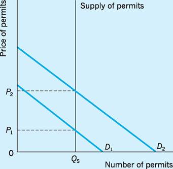
Fig. 10.5 Determining the market price for permits.

responsible for permits may issue Q_s permits. With demand for permits at D₁ the price will be set at P₁. If new polluters enter the market the demand for permits will increase, e.g. to D₂, and the equilibrium permit price will rise to P₂. If, for any reason, the agency wishes to relax the standard set, then more permits will be issued and the supply curve for per­mits will shift to the right. Alternatively, the standard could be tightened, by the agency purchasing permits on the open market from polluters, which would have the effect of shifting the supply curve to the left.

The EU Emissions Trading Scheme uses the idea of tradeable permits in seeking to reduce greenhouse gas emissions.

The EU Emissions Trading Scheme (ETS)

In the EU an Emissions Trading scheme (ETs) is being seen as a key economic instrument in a move to reduce greenhouse gas emissions. The ETs is intended to help the EU meet its commitments as part of the Kyoto Protocol. The EU took upon itself as part of the Protocol to reduce greenhouse gas emissions by 8% (from 1990 levels) by 2008-12. The idea behind the ETs is to ensure that those companies within certain sectors that are responsible for greenhouse gas emissions keep within specific limits by either reduc­ing their emissions or buying allowances from other organizations with lower emissions. The ETS is essen­tially aimed at placing a cap on total greenhouse gas emissions.

The emission of greenhouse gases is seen as a major cause of climate change, which has environ­mental and economic implications, not least in terms of floods and drought, and in October 2001 the European Commission proposed that an ETS should be established in the EU in order to reduce such emissions. The result is that an ETS, in the first instance covering only CO₂ emissions, commenced on 1 January 2005, representing the world’s largest mar­ket in emissions allowances. In the first phase, which ran from 2005 to 2007, the ETS covered companies of a certain size in sectors such as energy, production and processing of ferrous metals, the mineral indus­trial sectors and factories making cement, glass, lime, brick, ceramics, pulp and paper. In the larger Member States it has been estimated that between 1,000 and 2,500 installations will be covered, whereas in the other Member States the number could be between 50 and 400. In terms of the UK, this represents in the region of 1,500 installations, which emit approxi­mately 50% of the economy’s CO₂ emissions. The second phase, which is running from 2008-12, includes other sectors such as aviation. In the UK a number of government departments and agencies are responsible for issuing allowances (permits).

With the advent of the ETS an electronic registry system has been developed so that when a change in the ownership of allowances takes place there is a transfer of allowances in terms of the registry system accounts. This registry is similar to a banking clearing system that tracks accounts in terms of the ownership of money. In order to buy and sell the allowances each company involved in the scheme will require an account.

How will the Emissions Trading Scheme work?

This section details a hypothetical situation that will explain how emissions trading operates. In the fol­lowing analysis we assume there are two companies A and B each emitting 60,000 and 40,000 tonnes of CO₂ per annum respectively. Each company is represented in Fig. 10.6. The marginal abatement cost (MAC) curves refer to the extra cost to the firm of avoiding (abating) emitting the last unit of pollution. The MAC for company A increases more slowly than for company B as emissions are cut back, indicating that the cost of abatement is higher for company B than for company A.

With no controls on the level of emissions, the total level of CO₂ emissions will be 210,000 tonnes (120,000 tonnes from company A and 90,000 from company B). If we now assume that the authorities want to reduce CO₂ emissions by 50% (so that 105 million tonnes is the maximum) then this can be achieved by issuing 105,000 emission allowances each equal to 1 tonne. If they are issued on the basis of previous emission levels (‘grandfathering’) then company A would receive 60,000 emission allow­ances (or tradeable permits) and company B 45,000, based on one allowance representing the right to emit one tonne of CO₂. If this were the case then company A would have to reduce its emissions to 60,000 tonnes and company B to 45,000 tonnes. Based on this, company A would have a MAC of £1,200 and company B of £3,000. Given this situation, company B would buy permits if it could pay less than £3,000 for each, and company A would sell them for a price greater than £1,200. Company A would sell them, since the revenue earned from the sale would be

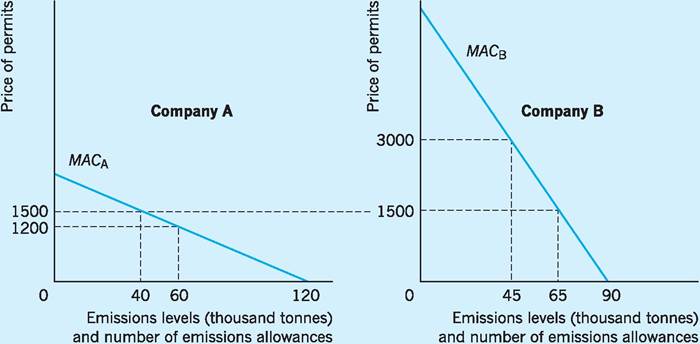
Fig. 10.6 Marginal abatement cost (MAC) and the trading in emissions allowances.

greater than the additional abatement cost incurred by reducing emissions. There is thus a basis for trade in emissions allowances and this will continue until the MACs are identical. In Fig. 10.6 this occurs at a price of £1,500 with 40,000 tonnes of CO₂ emitted by company A and 65,000 by company B, with com­pany A selling 20,000 emissions allowances to com­pany B. Overall the price of the allowances will be determined by supply and demand.

Potential advantages of the ETS

A number of potential advantages have been put forward in terms of the use of an ETS when dealing with issues such as the control of emissions affecting climate change, most notably the following.

■ Unlike pollution taxes, which begin by making com­panies pay for something they were once getting for free, emissions allowances begin by creating and distributing a new type of property right.

■ It is politically easier to get companies to agree on a pollution-control policy that begins by distribut­ing a valuable new property right (permit) than by telling them that they will have to pay a new tax. The reason for this is that the emissions allowance will have a market value as long as the number of allowances created is limited. In other words it is a more acceptable policy instrument for firms directly involved in the ETS.

■ Permits are cost-effective since they provide incen­tives for polluters with low abatement costs to abate (avoid) pollution and sell the permits they no longer require, while providing incentives for polluters with higher abatement costs to purchase these permits rather than abate. In other words a ready-made market exists.

■ According to the White Paper on the Future of Air Transport (Department for Transport 2003) one of the advantages of emissions trading is that it guarantees the desired outcome in a way not achieved by alternative market-based and non­market-based instruments, such as the introduc­tion of a charge (environmental tax). Companies have flexibility in that they can achieve their emis­sion reduction levels based on their own strategy, i.e. either by reducing emissions or by purchasing emissions allowances. Either way the desired envi­ronmental outcome is achieved, since the cap on overall emissions has been established.

Potential disadvantages of the ETS

The scheme came into force on 1 January 2005; how­ever, a number of potential disadvantages have also been pointed out.

■ An appropriate system of initially allocating the emissions allowances is all-important. In terms of the hypothetical situation outlined above, the allowances were allocated on the basis of current emissions, with companies A and B each receiving allowances representing half their emission levels. There are, however, difficulties with this, in that companies may already have successfully reduced their level of emissions and are now penalized for having done so by receiving less of the allowances. An alternative to this grandfathering approach could be to allocate allowances equally to those companies that are part of the ETS. This method also has inherent difficulties in that companies may differ in terms of the amount of pollution they cur­rently emit. In terms of the EU ETS, a mechanism closer to the former was adopted.

■ In terms of the philosophy underpinning the use of an emissions allowance scheme, it can be argued that it gives the owner of an allowance the right to pollute, in other words a permit to emit pollutants.

■ It is possible that a few polluters may purchase all the available permits, making it difficult for new companies to enter a particular sector. In this way allowances could act as a barrier to entry and thus be seen as anti-competitive. It has been stated, however, that the idea behind the ETS is to limit emissions and not to limit output. There is, however, a need to be aware of the potential diffi­culties new entrants to a sector may face.

■ Any scheme of this nature will have an administra­tion cost not least in terms of maintaining the electronic registry system. There is also a need to monitor the allowance transactions so that com­panies are emitting only what they are entitled to. If companies do not surrender allowances neces­sary to cover their annual emissions then they will be liable to a penalty, which in the first phase of the scheme will be ˆ40 per tonne of CO₂ emitted.

Conclusions

The EU ETS represented a new market-based ap­proach to dealing with the issue of CO₂ emissions and their related impacts on climate change. The scheme was introduced in the EU in January 2005 and is administered by a number of environmental bodies throughout the UK. The scheme has a number of potential advantages, notably the fact that it is establishing a new form of property right, it is more acceptable relative to pollution taxes, it is cost­effective and is flexible. There are, however, potential difficulties, not least in terms of allocating the emis­sions allowances, the ethical aspect of creating a right to pollute, the possibility of companies cornering the market in emissions allowances and the administra­tive costs. Overall, time alone will tell whether the ETS will be seen as a successful new market-based solution to the problem of greenhouse gas emissions.

In January 2008, the European Commission pro­posed a number of changes to the scheme, including centralized allocation (no more national allocation plans) by an EU authority, the auctioning of a greater share (60+ %) of permits rather than allocating them freely, and inclusion of other greenhouse gases, such as nitrous oxide and perfluorocarbons. These changes are to become effective from January 2013 onwards, i.e. in the 3rd Trading Period under the EU ETS. The proposed caps for the 3rd Trading Period foresee an overall reduction of greenhouse gases for the sector of 21% in 2020 compared to 2005 emissions. The EU ETS has recently been extended to the airline industry, but only after 2012.

Bargains

The idea here is that if we assign ‘property rights’ to the polluters giving them the ‘right to pollute’, or to the sufferers giving them the ‘right not to be polluted’, then bargains may be struck whereby pollution is curbed. For instance, if we assign these property rights to the polluters, then those who suffer may find it advantageous to compensate the polluter for agreeing not to pollute, the suggestion being that compensation will be offered by the sufferers as long as this is less than the value of the damage which would otherwise be inflicted upon them. Alternatively, if the property rights are assigned to the sufferers, who then have the ‘right’ not to be polluted, then the polluters may find it advantageous to offer the sufferers sums of money which would allow the polluters to continue polluting, the suggestion being that the polluters will offer compensation to the sufferers as long as this is less than the private benefits obtained by expanding output and thereby increasing pollu­tion. Under either situation, economists such as R. Coase have shown that clearly assigned property rights can lead to ‘bargains’ which bring about output solutions closer to the social optimum than would otherwise occur.

From Fig. 10.7 we can see that, with no regula­tion, the polluter will seek to maximize total net pri­vate benefits (profits) producing at Q_b, whereas Q_s is

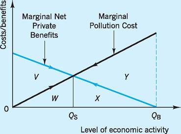
Fig. 10.7 Negotiation under property rights.

the social optimum. The introduction of property rights can, however, change this situation. If the pol­luter is given the property rights, then the sufferer will (provided polluter and sufferer have the same infor­mation!) find it advantageous to compensate/bribe the polluter to cease output at Q_s. For any extra out­put beyond Q_s the losses to the sufferer exceed the benefits to the polluter (e.g. X + Y > X at output Q_b). There is clearly scope for a negotiated solution at output level Q_s.

A similar negotiated outcome can be expected under the Coase theorem if the sufferer is given the property rights. This time the polluter will (given symmetry of information) find it advantageous to choose the socially optimum output Q_s and offer compensation equivalent to W to sufferers. For any extra output beyond Q_s, the gains to the polluter are more than offset by the (actionable) losses to the sufferers (e.g. X < X + Y at output Q_b). There is, again, clearly scope for a negotiated solution at output level Q_s.

The principle of ‘sufferer pays’ is already in evidence. For example, Sweden assists Poland with reducing acid rain because the acid rain from Poland damages Swedish lakes and forests. Similarly, the Montreal Protocol of 1987 sought to protect the ozone layer by including provisions by which China, India and other developing countries were to be compensated by richer countries for agreeing to limit their use of chlorofluo­rocarbons (CFCs). On this basis, Brazil has argued that it is up to the developed countries to compensate it for desisting from exploiting its tropical rainforests, given that it is primarily other countries which will suffer if deforestation continues apace.

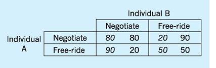
Fig. 10.8 Bargaining and game theory.

Bargaining, game theory and the free-rider problem

Chapter 6 (Oligopoly) introduced the idea of game theory, and we now apply this to the bargaining situation. Assume there are two sufferers from the pollution emitted from a factory. The two sufferers, individuals A and B, each have a level of utility equal to 50 utils. Individuals A and B are thinking about involving themselves in negotiation with the factory polluter. In reaching their decision there are four scenarios (Fig. 10.8).

1 Both individuals A and B decide not to negotiate with the polluter. The outcome is that both con­tinue to suffer and obtain a utility of 50 utils.

2 Both individuals A and B decide to negotiate with the polluter. There is a cost in negotiating which is equal to 70 utils each. If they negotiate together, however, they are likely to obtain major conces­sions, which could be equal to 100 utils for each individual. In this situation both individuals A and B benefit by a further 30 utils, resulting in each having utility of 80 utils.

3 Individual A decides to negotiate while B free-rides. In this situation the bargaining strength of the suf­ferers will be somewhat less and as such the gains from negotiation could be only 40 utils. In this situation the expected utility from negotiation for A would now be 20 utils (the original 50 utils plus the gain of 40 utils minus the cost of 70 utils). For individual B, however, the expected gain is 40 utils with no negotiation costs involved because of free­riding. Thus B’s expected utility is 90 utils.

4 Individual B decides to negotiate while A free-rides. In this situation A’s expected utility is 90 utils and B’s 20 utils.

Each individual has one of two options, either to negotiate or to free-ride. The left side of each box (in italics) refers to individual A’s outcomes (payoffs) and the right side to individual B’s outcomes (pay­offs). Taking a free-ride might seem an attractive option for each individual, yielding the highest payoff (90) in the belief that the other individual will indeed negotiate. However, if both decide to free-ride this essentially means both decide not to negotiate and the outcome is a less attractive payoff (50). The situation is the same as in the prisoner’s dilemma, which is also part of game theory (see Chapter 6).

If each selects the best outcome for itself inde­pendent of the reaction of the other, then each will choose to free-ride, believing it can achieve a payoff of 90 utils. This is the so-called ‘dominant strategy’ for the game, but in fact the outcome from following this strategy is only 50 utils each. Had each individual sought to negotiate rather than free-ride, then each would have been better off with 80 utils apiece. If sufferers are more likely to attempt to free-ride in this way, then giving them the property rights by making the polluter pay may be the best way of ensuring that the socially optimum bargaining outcome is achieved.

Non-market-based incentives: environmental standards and regulations

Environmental standards

Setting standards is a common option in terms of controlling pollution. For example, minimum stan­dards are set in terms of air and water quality and the polluter is then free to decide how best to meet the standard. A regulator then monitors the situation and action is taken against any polluter who fails to main­tain the standard set.

A standard St₁ could be set as illustrated in Fig. 10.9. This would achieve the optimum scale of economic activity Q_s and the optimum level of pollution. As with an environmental tax, standards require accurate information on MNPB and MEC. For example, the standard could be set at St₂ which would require a scale of economic activity equal to Q_a. This is not an optimum position since the mar­ginal net private benefits derived by the polluter Q_aX are greater than the marginal external costs Q_a Y. In other words, the standard is too severe.

In addition, in terms of Fig. 10.9 the penalty Pen₁ imposed on polluters who violate the standard set is not adequate. In fact, the polluter will be tempted to pollute up to Q_b since for each unit up to Q_b the

Fig. 10.9 Setting the appropriate standard and imposing the appropriate penalty.

penalty will be less than the profits received by the polluter, as measured by the MNPB curve. The pol­luter will not produce in excess of Q_b since for each unit beyond Q_b the penalty incurred would be greater than the profit obtained from that production. Of course, it is always possible that the pollution will go undetected and therefore no penalty will be imposed. With an optimal standard of St₁ the penalty should be Pen₂ and consistently enforced.

The setting of a standard such as St₁ will achieve the optimum level of economic activity and therefore pollution, provided that the penalty is set at Pen₂ and that this penalty is effectively enforced. Any ‘mistakes’ in the form of setting an inappropriate standard and/or an inappropriate penalty will lead to a misallocation of resources.

In the EU, a legally binding regulation on maxi­mum emissions of greenhouse gases by new vehicles comes into force in 2015, namely a maximum emis­sion of 130 grammes of CO₂ per kilometre travelled by new cars from that date. In the UK, the Environ­mental Protection Act (1989) laid down minimum environmental standards for emissions from over 3,500 factories involved in chemical processes, waste incineration and oil refining. The factories have to meet these standards for all emissions, whether into air or water or onto land. Factory performance is monitored by a strengthened HM Inspectorate of Pollution, the costs of which are paid for by the factory owners themselves. The Act also provided for public access to information on the pollution created by firms. Regulations were also established on restricting the release of genetically engineered bacteria and viruses and a ban was imposed on most forms of straw and stubble burning from 1992 onwards. Stricter regulations were also imposed on waste dis­posal operations, with local authorities given a duty to keep public land clean. On-the-spot fines of up to £1,000 were instituted for persons dropping litter.

Regulations have also played an important part in the five ‘Environmental Action Programmes’ of the EU, which first began in 1973. For example, specific standards have been set for minimum acceptable levels of water quality for drinking and for bathing. As regards the latter, regular monitoring of coastal waters must take place, with as many as 19 separate tests undertaken throughout the tourist season.

Of course regulations may be part of an integrated environmental policy which also involves market­based incentives. A tradeable permits system for sul­phur dioxide emissions has been long established in the US and works in tandem with the standards imposed by the US Clean Air Act.

We now review two key environmental issues to examine the relative merits of market-based and non­market-based incentives for dealing with environ­mental problems, namely global warming and transport-related pollution.

I Global warming

This refers to the trapping of heat between the earth’s surface and gases in the atmosphere, especially CO₂. Currently some six billion tonnes of CO₂ are released into the atmosphere each year, largely as a result of burning fossil fuels. In fact CO₂ constitutes some 56% of these ‘greenhouse gases’, with CFCs, used mainly in refrigerators, aerosols and air-conditioning systems, accounting for a further 23% of such gases, the rest being methane (14%) and nitrous oxide (7%). By trapping the sun’s heat, these gases are in turn raising global temperature (global warming). On present estimates, temperatures are expected to increase by a further 1 °C in the next two decades, when an increase of merely half a degree in world temperature over the past century is believed to have contributed to a rise of 10 cm in sea levels. Higher sea levels (resulting from melting ice caps), flooding and various climatic changes causing increased deserti­fication and drought have all been widely linked to global warming.

The whole debate on curbing emissions of CO₂ and other ‘greenhouse gases’ in an attempt to combat global warming usefully highlights a number of issues:

■ a non-zero level of pollution as socially efficient;

■ the respective advantages and disadvantages of market-based and non-market-based incentives in achieving socially efficient solutions.

We have already addressed some of the environ­mental implications of global warming. There are clearly significant social damage costs associated with emissions of CO₂, which rise at an increasing rate with the total level of emissions. This situation is represented by the Total Damage Costs curve in Fig. 10.10(a).

However, seeking to reduce CO₂ emissions will also impose costs on society. For instance, we may need to install expensive flue-desulphurization plants in coal-burning power stations, or to use (less effi­cient) sources of renewable energy (e.g. wind, wave, solar power). These various costs are represented by the Total Abatement Costs curve in Fig. 10.10(a). We might expect these Total Abatement Costs to rise at an increasing rate as we progressively reduce the level of CO₂ emissions, since the easier and less costly means of cutting back on CO₂ emissions are likely to have been adopted first.

In Fig. 10.10(a), we can see that the consequence of taking no action to reduce CO₂ emissions would leave us at Q_p, with zero abatement costs but high total damage costs.

What must be stressed here is the importance of seeking to identify both types of cost. On occasions, environmentalists focus exclusively on the damages caused by global warming, whereas producers con­cern themselves solely with the higher (abatement) costs of adopting less CO₂ intensive methods of production.

The analysis is simplified (Fig. 10.10(b)) by using marginal changes in the damage costs or abatement costs related to each extra tonne of CO₂ emitted or abated. The socially optimum level of CO₂ emissions is where marginal damage costs exactly equal mar­ginal abatement costs, i.e. output Q_s in Fig. 10.10(b). To emit more CO₂ than Q_s would imply marginal

Fig. 10.10 Using abatement and damage cost curves in finding a socially optimum level of pollution.

damage costs to society greater than the marginal cost to society of abating that damage. Society is clearly disadvantaged by any emissions in excess of Q_s. Equally, to emit less CO₂ than Q_s would imply marginal damage costs to society less than the mar­ginal cost to society of abating that damage. In this case society is disadvantaged by seeking to cut CO₂ emissions below Q_s.

Setting the targets

If we are to apply our analysis in practical ways we must seek to value both the marginal damage and the marginal abatement cost curves. Again we are faced with the conceptual problem of placing a valuation on variables to which monetary values are at present only rarely attached, if at all. In addition, in a full cost-benefit analysis we must select a rate of discount (see Chapter 17) to enable a comparison to be made between effects in the distant future and the costs of policies introduced today.

Uncertainty will therefore clearly be involved in any attempt to evaluate the costs and benefits of policy action or inaction. The target for reducing CO₂ emissions (Q_p - Q_s in Fig. 10.10(b)) to the socially optimum level will clearly be affected by such uncer­tainty. Analysts often use ‘scenarios’ of high, medium and low estimates for marginal damage and marginal abatement cost curves. For instance, Nordhaus (1991) estimated each of these marginal cost curves for both CO₂ emissions and for the broader category of greenhouse gases, based on US data. His high estimate of marginal damage costs was calculated at $66.00 per tonne of CO₂, his low estimate at only $1.83 per tonne of CO₂. We can use Fig. 10.10(b), above, to illustrate this analysis. In the high estimate case, the marginal damage cost curve shifts vertically upwards, Q_s falls, and the ‘target’ reduction in CO₂ emissions (i.e. Q_s - Q_p) increases. On this basis, Nordhaus advocates reducing CO₂ emissions by 20%. It is hardly surprising (in view of the valuation discrepancy noted above) that in his low estimate case, the marginal damage cost curve shifts vertically downwards in Fig. 10.10(b), Q_s rises, and the target reduction in CO₂ emissions (i.e. Q_s - Q_p) falls. On this basis Nordhaus advocates reducing CO₂ emis­sions by only about 3%.

The Stern Committee Report in 2006 estimated higher marginal damage costs per tonne of CO₂ than even the high estimate case of Nordhaus. As a con­sequence, the target CO₂ emission for Stern, with a higher marginal damage cost curve in Fig. 10.10(b), is well below that of Nordhaus (Hof and Van Vuuren 2008). The Stern ‘optimum’ target turns out to be a peak CO₂ concentration of 540 parts per million, whereas that for Nordhaus is a much higher target of 750 parts per million (World Bank 2010).

Stern Report on climate change

The Stern Report on climate change was published in late 2006, and is widely regarded as the most authoritative of its kind. Its key findings included the following.

■ CO₂ in the atmosphere in about 1780, i.e. just before the Industrial Revolution, has been esti­mated at around 280 ppm (parts per million).

■ CO₂ in 2006, however, had risen significantly to 382 ppm.

■ Greenhouse gases (CO₂, methane, nitrous oxide etc.) in 2006, were even higher at 430 ppm in CO₂ equivalents.

Two key scenarios were identified in the Stern Report.

Do nothing scenario

■ Temperature rise of 2 °C by 2050.

■ Temperature rise of 5 °C or more by 2100.

The damage to the global economy of such climate change from the ‘do nothing’ scenario is an estimated reduction in global GDP per head (i.e. consump­tion per head) of between 5% and 20% over the next two centuries. This occurs via rising temper­atures, droughts, floods, water shortages and extreme weather events.

Intervene scenario

The Stern Report advocates measures to stabilize greenhouse gas emissions at 550 ppm CO₂ equiva­lents by 2050. This requires global emissions of CO₂ to peak in the next 10-20 years, then fall at a rate of at least 1-3% per year. By 2050 global emissions of CO₂ must be around 25% below current levels. Since global GDP is expected to be around three times as high as today in 2050, the CO₂ emissions per unit of global GDP must be less than one-third of today’s level (and sufficiently less to give the 25% reduction on today’s levels).

The Stern Report estimated the cost of stabiliz­ation at 550 ppm CO₂ equivalents to be around 1% of current global GDP (i.e. around £200bn). This expenditure will be required every year, rising to £600bn per annum in 2050 if global GDP is three times higher than it is today. Stabilization would limit temperature rises by 2050 to 2 °C, but not prevent them. Otherwise temperature rises well in excess of 2 °C are predicted - possibly as much as 5 °C by 2100. Even limiting temperature rises to 2 °C by 2050 will inflict substantial damages, especially in terms of flooding low-lying countries as the ice caps melt, but also via more extreme weather conditions in various parts of the world.

Co-operative solutions and regulations

The arguments in favour of co-operative solutions to problems such as global warming have led many to support some type of regulatory framework such as that embedded in the Kyoto Protocol (see below). We can review some of these arguments using Fig. 10.11, which represents a situation in which the benefits to a country, A, from pollution reduction accrue only partly to itself, the remaining (and more substantial) beneficiaries from A’s pollution reduction being the rest of the region (here the world) of which A is but a part. However, A is faced with having itself to pay the costs of any pollution reduction (abatement) it undertakes.

In Fig. 10.11 A_mb and A_mc are country A’s mar­ginal benefits and marginal costs of pollution reduc­tion (note that the horizontal axis is pollution reduction, so more pollution reduction in Fig. 10.11 - moving left to right - is the same as less pollution emission - moving right to left - in Fig. 10.10(b) above), whilst K_mb is the whole region’s (rest of the world’s) marginal benefit from country A’s pollution reduction.

Note that the maximum net benefit for the whole region (MW0) occurs with pollution reduction by country A of P_r. But the maximum net benefit for country A (LV0) occurs with pollution reduction by country A of only P_a. To induce A to undertake pollution reduction beyond P_a is in the best interest of

Fig. 10.11 Regional reciprocal pollution and the need for negotiation.

the whole region (world), but any further reduction in pollution by A beyond P_a brings extra benefit to itself only up to X (area VXP_a), and this is insufficient to cover its additional costs. In other words, A will require extensive compensation to induce it to reduce pollution to P_R or at least a regulatory framework in which A can recognize benefits to itself from other countries also acting with a regional or global per­spective in mind, rather than merely their own self­interest. It was in an attempt to provide such a global perspective for pollution reduction that the Kyoto Protocol was signed in 1997.

I Kyoto Protocol

Provisionally agreed in December 1997 via the UN Framework Convention on Climate Change, the main features of the Kyoto Protocol are as follows.

■ Developed countries to collectively reduce 1990 emission levels of six greenhouse gases by 5% by 2012.

■ Individual country targets to be set within this average.

■ Penalties for non-compliance.

■ Emissions trading to be allowed (via permits).

■ ‘Clean Development Mechanisms’ to be applied by which greenhouse gas reductions in develop­ing countries resulting from investments by developed countries can be credited to those developed countries, thereby reducing the pollu­tion reduction targets set for them in the Kyoto agreement.

To ratify the Kyoto Protocol needs the signatures of countries responsible for at least 55% of 1990 emissions of greenhouse gases. An initial problem was the unwillingness of the US to ratify the protocol, given that it alone represented some 35% of 1990 greenhouse gas emissions. Only in 2003 was the Kyoto Protocol provisionally ratified with the initial reluctance to ratify of Russia (18% of 1990 emis­sions), Canada and some other countries finally being overcome. Having a major source of greenhouse gas emissions such as the US outside the Kyoto Protocol is clearly a weakness for this co-operative approach to tackling global warming.

Copenhagen Accord

The Copenhagen Accord was an outcome of the December 2009 meeting of the UN Framework Convention on Climate change (UNFCCC). It sought to quantify responses required if increases in global temperature are to be kept below 2 °C by 2050, i.e. specified actions, targets, verification mechanisms, financing proposals. Nations were to submit these within a tight deadline within two months of the meeting. Many had seen Copenhagen as an oppor­tunity to put a more effective mechanism than Kyoto into the international arena, especially since Kyoto was seen by many to have neglected the developing countries, despite 52% of emissions now coming from the developing countries and 97% of the growth in greenhouse gas emissions by 2050 expected to come from these countries.

In the event, while over 102 countries had responded within the time limit, with national plans for targeted actions by 2020, covering over 80% of global emissions, these voluntary and rather ‘patch­work’ outcomes were seen by many as having failed to provide an effective successor to Kyoto. Never­theless, seven of the major developing countries (Brazil, China, India, Indonesia, South Korea, Mexico, South Africa) did provide specific emission reduction targets by 2020, despite the Accord not making such quantitative targets a compulsory requirement! China will seek to reduce CO₂ emissions per unit of GDP by 40-45% by 2020 as compared to the 2005 levels.

Achieving the targets

Whatever the targets set for reduced emissions, which policy instruments will be most effective in achieving those targets? The discussion by Ingham and Ulph (1991) is helpful in comparing market and non­market policy instruments. Many different methods are available for bringing about any given total reduction in CO₂ emissions. Users of fossil fuels might be induced to switch towards fuels that emit less CO₂ within a given total energy requirement. For instance oil and gas emit, respectively, about 80% and 60% as much CO₂ per unit of energy as coal. Alternatively, the total amount of energy used might be reduced in an attempt to cut CO₂ emissions.

Another issue is whether we seek to impose our target rate of reduction for CO₂ emissions on all sectors of the UK economy. For example, some 40% of CO₂ emissions come from electricity generation, 20% from the industrial sector and around 20% from the transport sector. Should we then ask for a uni­form reduction of, say, 25% across all sectors? This is unlikely to be appropriate, since marginal abate­ment cost curves are likely to differ across sectors and, indeed, across countries. For instance, it has been estimated that to abate 14% of the air pollution emitted by the textiles sector in the USA will cost $136m per annum. However, to abate 14% of the air pollution emitted by each of the machinery, electrical equipment and fabricated metals sectors will cost $572m, $729m and $896m respectively (World Bank 1992). As well as differing between industrial sectors within a country, abatement costs will also differ between countries. For example, it has been estimated that a 10% reduction in CO₂ emissions by 2010 (as compared to 1988 emission levels) will cost ˆ400 per tonne of CO₂ abated in Italy, but only ˆ200 per tonne abated in Denmark, and less than ˆ20 per tonne abated in the UK, France, Germany and Belgium (Commission of the European Communities 1992).

This point can be illustrated by taking just two sectors in the UK - say, electricity generation and transport - and by assuming that they initially emit the same amount of CO₂. Following Ingham and Ulph (1991) suppose that the overall target for reduc­ing CO₂ emissions is the distance O'O in Fig. 10.12.

We must now decide how to allocate this total reduction in emissions between the two sectors. In Fig. 10.12 we measure reductions in CO₂ emissions in electricity generation from left to right, and reduc­tions in CO₂ emissions in transport from right to left. Point A, for example, would divide the total reduction in emissions into OA in electricity gener­ation and O'A in transport. A marginal abatement cost (MAC) curve is now calculated for each sector. In Fig. 10.12 we draw the MAC curve for electricity generation as being lower and flatter than that for transport. This reflects the greater fuel-switching possibilities in electricity generation as compared to transport, both within fossil fuels and between fossil and non-fossil (solar, wave, wind) fuels. In other words, any marginal reduction in CO₂ emissions in electri­city generation is likely to raise overall costs by less in electricity generation than in transport. In transport there are far fewer fuel-substitution possibilities, the major means of curbing CO₂ emissions in transport being improved techniques for energy efficiency or a switch from private to public transport.

Fig. 10.12 Finding the ‘efficient' or ‘least-cost' solution for reducing CO₂ emissions in a two-sector model.

Given these different MAC curves for each sector in Fig. 10.12, how then should we allocate our reduc­tion between the two sectors? Clearly we should seek a solution by which the given total reduction in emis­sions is achieved at the least total cost to society: we shall call this the efficient or least-cost solution. In Fig. 10.12, this will be where marginal abatement costs are the same in both sectors, i.e. at point B in the diagram. We can explain this by supposing we were initially not at B, but at A in Fig. 10.12, with equal reductions in the two sectors. At point A, marginal abatement costs in transport are AC but marginal abatement costs in electricity generation are only AF. So by abating CO₂ by one more tonne in electricity generation and one less tonne in transport, we would have the same total reduction in CO₂ emis­sions, but would have saved CF in costs. By moving from point A to the ‘efficient’ point B, we would save the area CFE in abatement costs.

It follows, therefore, that for any given target for total reduction in CO₂ emissions, ‘efficiency’ will occur only if the marginal cost of abatement is the same across all sectors of the economy (and indeed across all methods of abatement). Pollution control policies which seek to treat all sectors equally, even where marginal abatement costs differ widely between sectors, may clearly fail to reach an ‘efficient’ solution.

Policy implications

We have previously seen that environmental policy instruments can be broadly classified into two types: market-based and non-market-based. Market-based policy instruments would include setting a tax on emissions of CO₂ or issuing a limited number of per­mits to emit CO₂ and then allowing a market to be set up in which those permits are traded. Non-market- based policy instruments would include regulations and directives. For example, in the UK, the Non­Fossil Fuel Obligation currently imposed on priva­tized electricity companies requires them to purchase a specified amount of electricity from non-fossil fuel sources.

We can use Fig. 10.12 to examine the case for using a tax instrument (market-based) as compared to regulation (non-market-based). A tax of BE on CO₂ emissions would lead to the ‘efficient’ solution B. This is because polluters have a choice of paying the tax on their emissions of CO₂ or of taking steps to abate their emissions. They will have an incentive to abate as long as the marginal cost of abatement is lower than the tax. So electricity generating com­panies will have incentives to abate to OB, and trans­port companies to O'B, in Fig. 10.12 above. Since every polluter faces the same tax, then they will end up with the same marginal abatement cost. Here ‘prices’, amended by tax, are conveying signals to producers in a way which helps coordinate their (profit maximizing) decisions in order to bring about an ‘efficient’ (least cost) solution.

The alternative policy of government regulations and directives (non-market-based instruments) in achieving the ‘efficient’ solution at B in Fig. 10.12 would be much more complicated. The government would have to estimate the MAC curve for each sector, given that such curves differ between sectors. It would then have to estimate the different percentage reductions required in each sector in order to equalize marginal abatement costs (the ‘efficient’ solution). It is hardly reasonable to suppose that the govern­ment could achieve such fine tuning in order to reach ‘efficient’ solutions.

The market-based solution of tax has no adminis­trative overhead. Producers are simply assumed to react to the signals of market prices (amended by taxes) in a way which maximizes their own profits. Regulations, on the other hand, imply monitoring, supervision and other ‘bureaucratic’ procedures. Ingham and Ulph (1991) found that using a tax policy, as compared with seeking an equal propor­tionate reduction in CO₂ emissions by regulations, resulted in total abatement costs being 20% lower than they would have been under the alternative regulatory policy.

In a simulation by Cambridge Econometrics (Cowe 1998), a ‘package’ of seven green taxes, including a carbon tax based on industrial and commercial energy use, was estimated as cutting CO₂ emissions by 13% on 1990 levels by 2010. Rather encourag­ingly, this package of green taxes was estimated as raising a further £27bn in tax revenues by 2010, which could be used to cut employers’ national insur­ance by 3%, leading to almost 400,000 extra jobs. Only a small (-0.2%) deterioration was predicted for the balance of payments and for inflation (prices rising by 0.5%) by 2010 and GDP was even predicted to have received a small boost (+ 0.2%) by this package of green taxes. Such simulation studies are useful in that they ‘model’ impacts of tax measures throughout the economy, although one must carefully check the assumptions which underlie the equations used in computer models.

The Climate Change Levy

In the 1999 UK Budget, the Chancellor, Gordon Brown, announced that a Climate Change Levy (CCL) would be imposed on business use of energy from April 2001. The CCL is a tax applying to fossil fuel used by non-domestic (mainly commercial and industrial) users, applying at different rates to different fossil fuels. The rates are 0.42p per kWh for electricity, 0.15p per kWh for gas and 1.17p per kilogram for coal. Fuel oils are not liable for CCL as they are already liable for separate duty. The CCL is a revenue­neutral tax, meaning that the revenue produced by the tax will be recycled to companies so that for industry as a whole there will be no net increase in taxation. The revenues are recycled through a reduction of 0.3% in employers’ national insurance contributions, an increase in tax allowances for cer­tain energy-saving investments by a company, and payments from an energy-efficient fund for small and medium-sized companies. Certain large polluters are able to enter into negotiated voluntary agreement with the government to reduce energy consumption in exchange for a reduction (up to 80%) of CCL. Note that the tax does not apply to domestic energy use, although households will bear some of the bur­den of this tax in so far as firms pass the tax forward.

Critics have suggested that a carbon tax which was based solely on CO₂ content would be preferable, since the energy content of fuel does not necessarily reflect its carbon content. However, an energy tax is believed to be simpler to administer, being applied at a uniform rate per kilowatt-hour for all ‘primary’ fuels (coal, gas, oil), rather than a more complex differential rate depending on their carbon content.

I Conclusion

The World Bank has concluded that ‘regulatory poli­cies, which are used extensively in both industrial and developing countries, are best suited to situations that involve a few public enterprises and non-competitive private firms’ (World Bank 1992). It also concludes that economic incentives, such as charges, will often be less costly than regulatory alternatives. For instance, to achieve the least-cost or efficient solution of point B in Fig. 10.12 is estimated as costing some 22 times more in the US if particulate matter is abated by regulations, rather than by using market-based instruments. Similarly, achieving this least-cost solu­tion by regulating sulphur dioxide emissions in the UK is estimated as costing between 1.4 and 2.5 times as much as achieving it by using market-based instru­ments. Certainly there has been considerable support for using tradeable permits as a key mechanism for tackling the emissions of CO₂ and other greenhouse gases as, for example, with the introduction of an Emissions Trading System by the EU in 2005.

However, regulatory policies are particularly appropriate when it is important not to exceed certain thresholds, e.g. emissions of radioactive and toxic wastes. In these cases, it is clearly of greater concern that substantial environmental damage be avoided than that pollution control be implemented by policies which might prove to be more expensive than expected. However, where the social costs of environmental damage do not increase dramatically if standards are breached by small margins, then it is worth seeking the least-cost policy via market incentives rather than spending excessive amounts on regulation to avoid any breach at all.

With market-based policies, all resource users or polluters face the same price and must respond accordingly. Each user decides on the basis of their own utility/profit preferences whether to use fewer environmental resources or to pay extra for using more. On the other hand, with regulations it is the regulators who take such decisions on the behalf of the users, e.g. all users might be given the same limited access to a scarce environmental resource. Regulators are, of course, unlikely to be well informed about the relative costs and benefits faced by users or the valuations placed on these by such users.

Market-based policies have another advantage, namely that they price environmental damage in a way which affects all polluters, providing uniform ‘prices’ to which all polluters can respond (see Fig. 10.12), thereby yielding ‘efficient’ or ‘least cost’ solutions. By contrast, regulations usually affect only those who fail to comply and who therefore face pen­alties. Further, regulations which set minimizing standards give polluters no incentives to do better than that minimum.

Our review of environmental concerns and possible remedial policies has, of necessity, been selective. We have considered the competing claims of market- and non-market-based incentives towards achieving socially efficient solutions. Market-based incentives often help avoid the necessity of external bodies seek­ing to evaluate marginal abatement cost and marginal damage cost curves. This is certainly an advantage in an area where such valuations are notoriously difficult. Nevertheless, there are situations where regulations, or a judicious mix of markets and regula­tions, may be the most appropriate way forward. In any case, all the interdependences of any proposed solution must be fully taken into account before any final decisions are made. What is beyond dispute is that the environment and the economic system are highly interrelated, and neither can be considered in isolation from the other.

Key points

■ The environment interacts with the cir­cular flow, providing amenity services, natural resources and the assimilation of waste products.

■ An ‘Index of Sustainable Economic Welfare’ (ISEW) adjusts the conventional GNP figure for environmental impacts. On this basis, the growth of ISEW per head for the UK in the period 1950-2005 was a mere 0.5% per annum, much less than the growth in real GNP per head of 2.0% per annum over the same period.

■ The optimum level of pollution for soci­ety is unlikely to be zero. Rather it will occur at the (positive) level at which marginal damage costs exactly equal marginal abatement costs.

■ Assessing such an optimum involves find­ing solutions to problems of valuation of environmental impacts, especially where no market prices exist.

■ Policy instruments which might be used to achieve a social optimum include both market-based incentives (taxes, tradeable permits and negotiation) and non-market- based incentives (various standards and regulations).

■ There is evidence to suggest that in most cases a given objective can be achieved at least cost by a combination of market­based policy instruments.

■ Considerable emphasis is now being placed on tradeable permits as a market­based system for tackling greenhouse gas emissions.

■ Where the benefits of pollution reduc­tion measures extend beyond the country concerned, there is a case for co-operative and international agreements along the lines of the Kyoto Protocol if socially optimum outcomes are to be achieved.

■ The Copenhagen Accord is an attempt to develop specific national action plans to keep global warming within 2 °C of current temperatures by 2050.

Now try the self-check questions for this chapter on the Companion Website. You will also find useful links to relevant websites.

References and further reading

Berck, P. and Helfand, G. (2010) Economics of the Environment, Harlow, Pearson Education.

Bergstrom, J., Russell, R. and Randall, A. (2010) Resource Economics: An Economic Approach to Natural Resource and Environmental Policy (3rd edn), Cheltenham, Edward Elgar. Commission of the European Communities (1992) The climate challenge, economic aspects of the Community’s strategy for limiting CO₂ emissions, European Economy, 51, May. Cowe, R. (1998) Green taxes come up against pain barrier, Guardian, 2 February. Department for Transport (2003), The Future of Air Transport, Cm 6046, December, London, The Stationery Office.

Hof, A. and Van Vuuren, D. (2008) Analysing the costs and benefits of climate policy: value judgements and scientific uncertainties, Global Environmental Change, 18(3): 412-24. Ingham, A. and Ulph, A. (1991) Economics of global warming, Economic Review, 9(2): 2-6. Ison, S., Peake, S. and Wall, S. (2002) Environmental Issues and Policies, Harlow, Financial Times/Prentice Hall.

Jackson, T. and Marks, N. (1994) Measuring Sustainable Economic Welfare - A Pilot Index: 1950-1990, Stockholm Environment Institute.

Jackson, T., Marks, N., Ralls, J. and Stymne, S. (1997) Sustainable Economic Welfare in the UK 1950-1996, London, New Economics Foundation.

Kerry Turner, R., Pearce, D. and Bateman, I. (1994) Environmental Economics, Hemel Hempstead, Harvester Wheatsheaf.

Lawrence, P. (2002) Can the World Bank rescue Africa’s economies?, Economic Review, 19(4): 20-4.

Lubin, D. and Esty, D. (2010) The sustainability imperative, Harvard Business Review, May, 89-99.

Maddison, D., Pearce, D. et al. (1996) Blueprint 5: The True Costs of Road Transport, London, Earthscan Publications Ltd.

Markandya, A. and Mason, P. (1999) Air pollution and health, Economic Review, 17(2): 2-4.

Newbery, D. M. (1995) Economic effects of (18th Report) recommendations, Economic Journal, 105(September): 1258-72.

Nordhaus, W. (1991) To slow or not to slow: the economics of the greenhouse effect, Economic Journal, 101(407): 920-37

O’Doherty, R. (1994) Pricing environmental disasters, Economic Review, 12(1).

ONS (2003) UK Environmental Accounts 2003, London, Office for National Statistics.

Palmer, A. (2001) Organic food, Economic Review, 19(1): 2-5.

Pearce, D. (1991a) Towards the sustainable economy: environment and economics, Royal Bank of Scotland Review, 172(December): 3-15. Pearce, D. (1991b) Economics and the environment, Economics, Journal of the Economics Association, 27(1): 113.

Pearce, D. (1998) Sustainable development: taking stock for the future, Economic Review, 16(1): 4-7. Sheppard, P. and Walter, M. (2002) The Dibden Bay project: a matter of choice, Economic Review, 19(4): 25-9.

Stern, N. (2007) The Economics of Climate Change: The Stern Review, Cambridge, Cambridge University Press.

Tietenberg, T. and Lewis, L. (2008) Environmental and Natural Resource Economics (8th edn), Harlow, Financial Times/Prentice Hall. Tietenberg, T. and Lewis, L. (2009) Environmental Economics and Policy (6th edn), Harlow, Financial Times/Prentice Hall. Turner, K. (1991) Environmental economics, Developments in Economics: an Annual Review, 7. Unruh, G. and Ettenson, R. (2010a) Growing green, Harvard Business Review, June, 94-100. Unruh, G. and Ettenson, R. (2010b) Winning in the green frenzy, Harvard Business Review, November, 110-15.

Willis, K. (1991) The priceless countryside: the recreational benefits of environmental goods, Royal Bank of Scotland Review, 172(December): 34-8.

World Bank (1992) World Development Report 1992: Development and the Environment, Washington DC.

World Bank (1994) World Development Report 1994: Infrastructure for Development, Washington DC.

World Bank (2010) World Development Report 2010: Development and Climate Change, Washington DC.