Robustness: basic stuff

The rest of this chapter is essentially about the robustness of the findings reported in Table 1. In this section I start out with a set of relatively straightforward and somewhat plodding robustness checks.

3.1. Depreciation rate

The effect of varying the depreciation rate in the perpetual-inventory calculation is to change the relative weight of old and new investment. A higher rate of depreciation will increase the relative capital stock of countries that have experienced high investment rates towards the end of the sample period. Poorer countries have in general experienced a larger increase in investment rates over the sample period, but the relative gain is very small, so it is unlikely that higher or lower depreciation rates will have a considerable impact on our calculation.^[382] In Figure 1 I compute and plot success₁ and success₂ for different values of S. Clearly, the sensitivity of the factor-only model to changes in S is minimal.

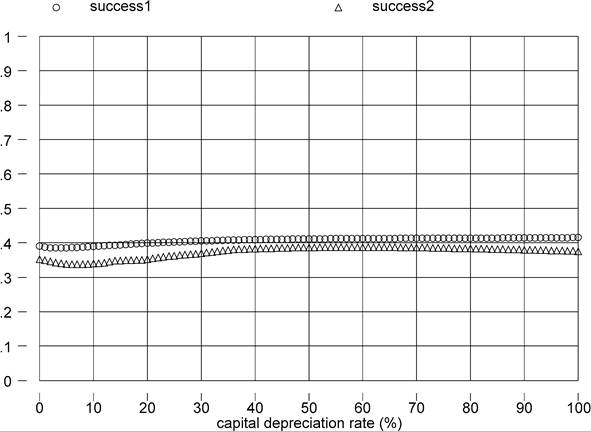
Figure 1. Depreciation rate and success.

3.2. Initial capital stock

The capital stocks in our calculations depend on the time series of investment (observ­able) and on assumptions on the initial capital stock, K₀, which is unobservable. Does the initial condition for the capital stock matter? One way to approach this question is to compute the statistic

i.e. the surviving portion of the guessed initial capital stock as a fraction of the final estimate of the capital stock.

A first check on this problem is to focus on a narrower sample with longer investment series. If we focus only on the 50 countries with complete investment data starting in 1950, we should be fairly confident that the initial guess plays little role in the value of the final capital stock. In this smaller, and probably more reliable, sample we get success₁ = 0.39, and success₂ = 0.48. Hence, the ratio of log-variances is unchanged relative to the full 94-country sample, but the inter-percentile ratio shows a considerable improvement. Clearly, though, as the sample size declines the inter-percentile ratio be­comes less compelling as a measure of dispersion, so on balance these results - though inconclusive - are reasonably reassuring.^[384]

Another strategy is to attempt to set an upper bound on the measures of success, by making extreme assumptions on the degree to which the capital stock in poor countries is mismeasured.

Another experiment is to estimate the initial capital stock by assuming that the factor- only model adequately explained the data at time 0. Suppose that we trusted the estimate K₀ = I₀/(g + 5) for the United States (where date 0 is 1950), and consequently for all other dates. Then for any other country we could estimate K₀ by solving the expression

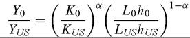
where 0 is now the first year for which both this country’s and the US' data on in­vestment, GDP, and human capital is available. Note that everything is observable in this equation except K0 (tough this does require us to construct new estimates of the human-capital stock for years prior to 1996). Clearly this procedure implies enormous variance in K₀, and this variance should persist to 1996, giving the factor-only model a real good shot at explaining the data. On the full sample this yields success₁ = 0.41 and success₂ = 0.34, and on the sub-sample with complete I data starting in 1950 it yields success ₁ = 0.45 and success₂ = 0.48.

3.2. Education-Wageprofile

By assuming decreasing aggregate returns to years of schooling the Hall and Jones method dampens the variation across countries in human capital, thereby potentially increasing the role of differences in technology. More generally, our measure of human capital may obviously be quite sensitive to the parameters of the function φ(s).

One way of checking this is to assume a constant rate of return, or φ(s) = φ_ss, and experiment with various values of the (constant) return to schooling φ_s. Since countries with higher per-capita income have higher average years of education, the factor-only model will be the more successful the steeper is the education-wage profile. Figure 2 confirms this by plotting success ₁ and success₂ as functions of φ_s.

While higher assumed returns to an extra year of education do lead to greater ex­planatory power for the factor-only model, only returns that are implausibly large lead to substantial successes. For success₁ (success₂) to be 0.75 the return to one year of school-

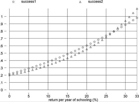
Figure 2. Returns to schooling and success.

ing would have to be around 25% (26%). As already mentioned, in the Psacharopoulos (1994) survey the average return is about 10%. The highest estimated return is 28.8% (for Jamaica in 1989), but this is a clear outlier since the second-highest is 20.1% (Ivory Coast, 1986). These tend to be OLS estimates. Instrumental variable estimates on US data are 17-20 percent at the very highest [Card (1999)] - sufficient for our measures of success to just clear the 50 percent threshold.

3.3. Years of education 1

De la Fuente and Domenech (2002) survey data and methodological issues that arise in the construction of international educational attainment data, such as the average years of education in the Barro and Lee data set. Their conclusion - perhaps not surprisingly - is that such series are rather noisy, and that this explains in part why human-capital based models often perform rather poorly. For several OECD countries they also construct new estimates that take into account more comprehensive information than is usually exploited, and find that for this restricted sample their measure substantially improves the empirical explanatory power of human capital.

To see if incorrect measurement of s is a likely culprit for the lack of success of the factor-only model, I compute our success statistics for the sub-sample covered in the De la Fuente and Domenech (2002) data set, first with our baseline data, and then with the new figures provided by these authors (in their Appendix 1, Table A.4) for 1995. This data is available for only 15 of our 94 countries. In this 15-country sample, with our baseline (Barro and Lee) schooling data, I obtain success₁ = 0.487 and succeess₂ = 0.976. In the same sample with the De la Fuente and Domenech data success₁ = 0.490 and success₂ = 0.977. The differences seem small.

This result is not particularly surprising because De la Fuente and Domenech (2002) show that the discrepancies between their measures and the ones in the literature are (1) stronger in first differences than in levels; and (2) stronger at the beginning of the sample than at the end.

3.4. Years of education 2

So far we have used Barro and Lee’s data on years of schooling in the population over 25 years old. This may be appropriate for rich countries with a large share of college graduates. But it is much less appropriate for the typical country in our sample. Barro and Lee (2001) also report data on years of schooling for the population over 15 years of age. These data can be combined with the data on the over-25 as follows.

First, note that we can write

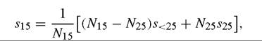
where s₁₅ and s₂₅ are the average years of education in the population over 15 and over 25 years of age, respectively (the data), and son these other φ s, we'll see that this assumption may actually be quite realistic. If we make the additional “steady state” assumption that h_t = h, we can write

and plugging this into (3) we get:

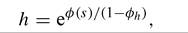
Note that this formulation magnifies the impact of differences in years of schooling, the more so the larger the elasticity of student human capital to teacher's human capital.

I continue to choose α = 1/3, and the Iirnction φ(∙) as described in Section 2. The new, unknown parameter is φ_h. In Figure 6 I plot successι and success₂ as functions of

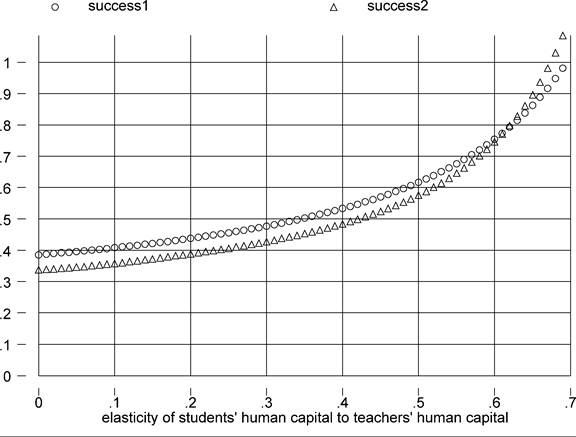
Figure 6. φh and success.

this parameter. Note that φ_h = 0 is the baseline case of Section 2. At the low values of φ_h implied by the baseline case the success measures are fairly insensitive to changes in the elasticity of students’ to teachers’ human capital. However, the relationship between the success measures and φ_h is sufficiently convex that when φ_h is 69% success is complete. Coincidentally, 69% is very close to the upper bound of the range of values Bils and Klenow consider “admissible” for φ_h (67%), though clearly this admissibility is purely theoretical: their preferred values are actually in the 0-20% range.^[391]

One way to think about what is reasonable for φ_h is to compute by how much the teachers’ human capital effect “blows up” the Mincerian return: from Equation (8) we see that with φ_h = 0.2 the “social” return to schooling is 1.2 times the private one; with φ_h = 0.4 it is 1.7 times larger; and with φ_h = 0.67 it is 3 times more. While it is hard to reach a firm conclusion, it would seem that reasonable priors on φ_h are inconsistent with large improvements in the fit of the factor-only model.

Turning to possible objective estimates of φ_h, the first option is of course to look for estimates of the effect of teachers’ years of education on student achievement. This is because under our assumptions differences in teacher’s quality are ultimately de­termined by teachers’ years of education. However, Hanushek’s (2004) review of the literature concludes that teachers’ measurable credentials - including years of educa­tion - have no measurable impact on schooling outcomes.^[392]

Another way to formulate priors on the possible magnitude of φh is to look at evi­dence on the effect of parental education on wages. After all, our simple representative­agent model of human capital is not explicit about the particular way the economy’s average level of human capital enhances the learning experience of new members of society. We can legitimately re-interpret h_t, therefore, as the human capital of parents. One recent set of log-wage regressions including the schooling of parents (alongside with an individual’s own schooling) is presented in Altonji and Dunn (1996). Depend­ing on data sources, and on whether the regression is estimated for men or women, their coefficient on father’s years of schooling ranges from -0.5% to 1%, and the co­efficient on mother’s schooling from less than 0.1% to about 0.5%. Note that given our functional form assumption the coefficient of parental education is φ_sφ_h, where φ_s is the return to own years of schooling (assumed constant for simplicity). If the return to own schooling, φ_s, is in the ball park of 0.10 (as the evidence on Mincerian coefficients roughly implies), and we focus on Altonji and Dunn’s upper bound of 0.01 for φ_sφ_h, we conclude that φ_h cannot be more than 0.1. A quick check with Figure 6 reveals that even this upper bound does not support a meaningful boost in the explanatory power of overall human capital.^[393]

3.5.1. Pupil-teacher ratios

The term h^φh in Equation (7) does not appear to enhance the success of the factor- only model. I now consider the term p^φp. Lee and Barro (2001) report data on the pupil-teacher ratio in a cross-section of countries for various periods since 1960, and separately for primary and secondary schooling. For each country, I focus on the pupil­teacher ratio in the years when the average worker attended school. To pinpoint this year, I need to start with an estimate of the age of the average worker, which I construct from LABORSTA.^[394] Then I assume that children begin primary schooling at the age of 6. This implies that the relevant observation for the primary pupil-teacher ratio would be for the year 1996-age + 6. Furthermore, using unpublished panel data by Barro and Lee on the duration of primary and secondary schooling, we can determine the relevant ob­servation for the secondary pupil-teacher ratio as 1996-age + 6 + duration of primary school.

In order to combine the primary and secondary ratios in a unique statistic, I combine the duration of schooling data with our basic data on the average years of schooling of the population over 25 years of age, s, to determine what fraction of schooling time the average worker spent in primary, and what fraction in secondary school. I then construct p by simply averaging the primary and secondary teacher-pupil ratio using as weights the time spent in these two grades, respectively. At the end of all this, I have data on p for 87 of our 94 countries.^[395]

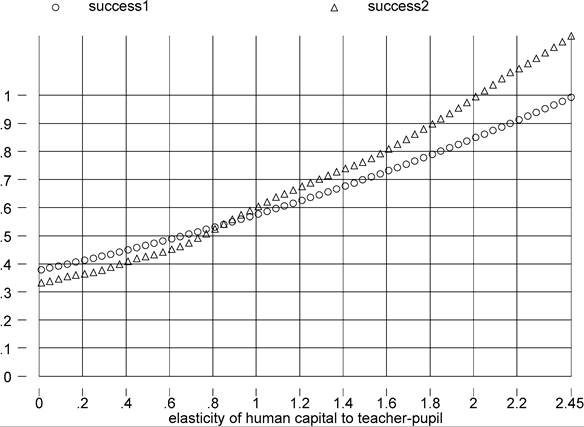
Figure 7. φp and success.

Figure 7 plots success₁ and success₂ as functions of φ_p. Since richer countries have higher teacher-pupil ratios, clearly a higher elasticity of human capital to this ratio implies a better fit, or greater success. What is a reasonable range of values for φ_p? At the low end of the spectrum there is the position taken by Hanushek and coauthors, who conclude that resources - including a large teacher-pupil ratio - have little if any effect on economic outcomes.^[396] At the other end of the spectrum, my own reading of the literature indicates that the highest published estimate of φ_p is a very sizable 0.5.^[397] However, even with this extremely high estimate it is clear that the fit of the model improves modestly, with our success measures barely attaining even the 50% mark.

3.5.2. Spending

I do not have direct data on materials, m and structures per student, k_h. Instead, I have - always from Lee and Barro (2001) - a measure of government spending per student in PPP dollars. The bulk of this spending typically goes to teacher salaries, so variation in these data also reflect differences in the number and possibly the quality of teachers per

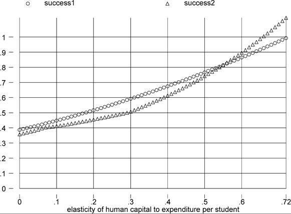
Figure 8. φ_sp and success.

student. However, to a certain extent, they may also reflect variation in materials. For the purposes of using these data, it seems sensible, therefore, to replace Equation (7) by A_h = spending^φsp, where the dating of the spending observation and the weights given to primary and secondary spending are determined as for the pupil-teacher ratio. For this exercise, I have data for 64 countries, and for this sample the measures of success are plotted in Figure 8. Again, rich countries devote more resources to education per student, so the fit of the model improves with φ_sp. However, again, there is the Hanushek position in the papers cited above, according to which φ_sp should be thought of as close to zero. At the other end of the range I have found an estimate of 0.2, which clearly is barely sufficient to even clear the 50% threshold of explanatory power.^29,30

4.2. Quality of schooling: test scores

Another way to investigate the potential of quality-of-education modifications to the basic model is to exploit information on the performance of students on reading, science,

²⁹ Johnson and Stafford (1973), who run a regression of log hourly wages on log state expenditure per student (and controls), obtaining a coefficient of 0.198. For the reasons discussed by Hanushek and co-authors there is a high presumption of upward bias in this estimate.

³⁰ Lee and Barro (2001) also report information on the duration of the schooling year (in days and hours), but these variables - while highly variable - are weakly, and if anything negatively, correlated with per-capita income, so that they are highly unpromising from the perspective of improving the fit of the model. Similarly, teacher salaries, as a percent of per-capita GDP, are higher in poorer countries.

and math tests in different countries. When students in one country outperform students of another (holding grade constant), we can assume that they have enjoyed schooling of higher quality, whether this higher quality comes from higher teacher-pupil ratios, quality of teachers, other expenditures, or other unobservables specific to the production of human capital. Hanushek and Kimko (2000) find that test scores enter significantly in growth regressions.

To implement this idea I think of A_h as a function of test scores: higher test scores signal higher human capital. Suppose, for example, that the relationship between school quality and test results is given by A_h = e^φττ, where τ is the test score.^[398] Then, with data on test scores, if we knew φ_τ we could construct a new counterfactual measure of óêí, or the output attributable to “observable” factors of production.

I use data on test scores provided by Lee and Barro (2001), who for several countries observe data on multiple tests (e.g.: math, science, and reading), and for multiple grades, at different dates. Ideally I would follow the procedure outlined in the previous sub­section, i.e. to “target” the year in which the average worker is presumed to have been in school. Because this data is very sparse, however, and mostly available in recent dates, I will focus on recent observations. This procedure is appropriate if the quality of education has grown over time at roughly similar rates across countries.

The two tests that afford the greatest country coverage - 28 countries with overlap­ping test, input, and output data - are a math and a science test imparted to 13-year-old children between 1993 and 1998. The scores are standardized on a 0-to-100 scale, and I take the simple average of the two test scores.^[399] With this summary measure of τ at hand, in Figure 9 I plot our measures of success against φ_τ.

The result should be treated with great caution given the very small sample size. Notice for example that, even for φ_τ = 0, both measures of success are considerably higher than in the full sample. With that caveat, it is true that students in rich countries perform better in standardized tests, and therefore the success of the model improves with φ_τ.

To find a benchmark for φ_τ against which to evaluate Figure 9, notice that our as­sumption on the relationship between test scores and school quality translates into an assumption on the relation between test scores and wages: a unit increase in test scores is associated with a φ_τ proportional increase in wages. I have chosen this exponential form because studies of the relationship between test scores and wages tend to report coefficients from regressions of log wages on absolute test scores. For example, the co­efficient φ_τ ? 100 (after rescaling the test data to be in the same units as ours) is reported to be between 0.08 and 0.34 by Murnane, Willett and Levy (1995); between 0.12 and 0.27 by Currie and Thomas (1999), and between 0.55 and 1.02 by Neal and Johnson (1996) - which is at the high end of the range of available estimates.^[400]

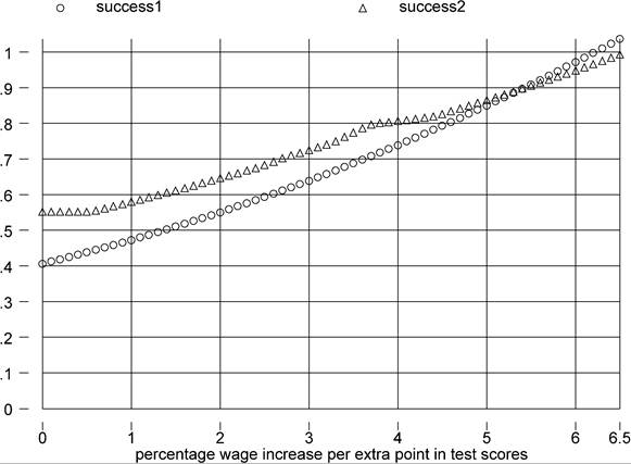
Figure 9. φ_τ(?100) and success.

Inspection of Figure 9 given this range of values suggests that using test scores as proxies for schooling quality cannot substantially improve the performance of the factor-only model. The problem is that, given the drastically reduced sample size, it is hard to take a stand on the degree to which this finding generalizes.

I can attain a slight increase in sample size if I drop the requirement that the tests be imparted in roughly the same period and roughly the same subject. If I use all the test considered, US data). Since the test results are reported to vary between 2 and 17 points, we assume that the test is on a 0-20 scale. When translated to our 0-100 scale this implies the φs reported in the text. The Currie and Thomas (1999) results imply that “students who score in the upper quartile of the reading exam earn 20% more than students who score in the lower quartile of the exam, while students in the top quartile of the math exam earn another 19% more. When they control for father’s occupation, father’s education, children, birth order, mother’s age, and birth weight, the wage gap between the top and bottom quartile on the reading exam is 13% for men and 18% for women, and on the math exam it is 17% for men and 9% for women” [Krueger (2003, p. 25)]. From here we can infer that φ_τ varies between 0.0012 and 0.0027 (dividing the percentage change in the wage by the 75 points that separate the top from the bottom quartile). Neal and Johnson (1996) run a regression of log real yearly wages on standardized AFQT test scores, and find a coefficient between 0.17 and 0.29. Introducing more controls the coefficients are between 0.12 and 0.16. Since the standard deviation of AFQT scores (as reported in the note to their Appendix A.3) is 36.65, this implies that a one-point increase in AFQT scores increases wages by between 0.33 and 0.79 percent. Given that AFQT scores range between 95 and 258, this implies a φ between 0.0055 and 0.0102 (treating each of the AFQT points as 1.64 of our 100 points). (Whether AFQT scores are measures of schooling outcome is somewhat controversial.) Hanushek and Kimko (2000) use essentially the same international test scores we are using here to explain the earnings of migrants to the US, and obtain φ_τ ? 100 of approximately 0.2.

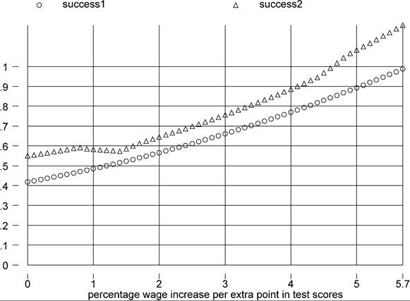
Figure 10. φ_τ (? 100) and success, all tests in the 90s.

scores available from the 1990s, i.e. I average across all tests irrespective of subject, age group, and specific year, our sample size becomes 42 and success is given by Figure 10. If I use all available tests, including those from decades before the 1990s, the sample size is 45 and success is shown by Figure 11. As we increase the sample size, the potential success of the factor-only model if anything declines.

4.3. Experience

Klenow and Rodriguez-Clare (1997) and Bils and Klenow (2000) also allow for differ­ences across countries in experience levels. Since Mincerian wage regressions indicate that experience increases earnings, it makes sense to correct human capital for the con­tribution of experience. This correction has two conflicting effects on the explanatory power of human capital. Since workers in rich countries live longer than workers in poor countries, this should boost rich countries' human capital. However, since rich­country workers spend more time in school, a smaller proportion of their time is spent accumulating experience, which reduces their relative human capital.^[401]

Klenow and Rodriguez-Clare (1997) find that the net effect is negative: experience is actually higher in poor countries. Hence, in their calculations correcting for experience lowers the explanatory power of the factor-only model. However, in order to compute

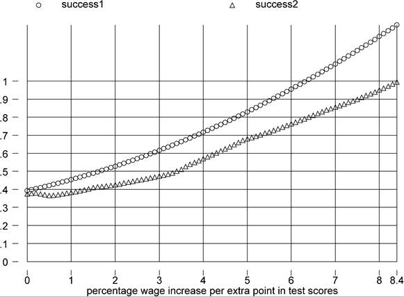
Figure 11. φ_τ (? 100) and success, all available test scores.

the average age of workers they rely on UN data on the age structure of the population, while in principle it would be more accurate to look at the age structure of the labor force. Using again the LABORSTA-based measure of the average age of the economi­cally active population in the formula

experience = age-schooling — 6,

I find that the correlation between experience and per-capita income is —0.29 in our 94-country sample. Therefore, I confirm the Klenow and Rodriguez-Clare conclusion that poor countries have less education but more experience. Adding experience to the factor-only model, therefore, will only worsen its explanatory power.^[402]

4.4. Health

Weil (2001) and Shastry and Weil (2003) point out that there are very large cross­country differences in nutrition and health status, and argue that these differences map into substantial differences in energy and capacity for effort. They find that accounting for health differences across countries increases by one-third the explanatory power of human capital for differences in per-capita income.

Weil (2001) uses as a proxy for health the Adult Mortality Rate (AMR), which mea­sures the fraction of current 15-year-old people who will die before age 60, under the assumption that age-specific death rates in the future will stay constant at current levels. In practice, this is a measure of the probability of dying “young”, and is therefore a plausible (inverse) proxy for overall health status.

The correction of human capital for health can be implemented through the assump­tion A_h = e^^amrAMR, where clearly φ_amr < 0: a higher adult mortality rate implies a less energetic workforce. I gather cross-country data on AMRs from the WDI, covering 92 of our 94 countries, for the year 1999. I plot success for different values of -φ_amr in Figure 12. Since richer countries have healthier workers, the explanatory power of human capital increases in -φ_amr.

Weil's preferred value for -φ_amr(? 100) is 1.68. Conditional on this value, I do con­firm his finding that the factor-only model's explanatory power improves considerably - indeed by almost one third, taking us well above the 50 percent threshold of success. This is therefore a very important and promising contribution.

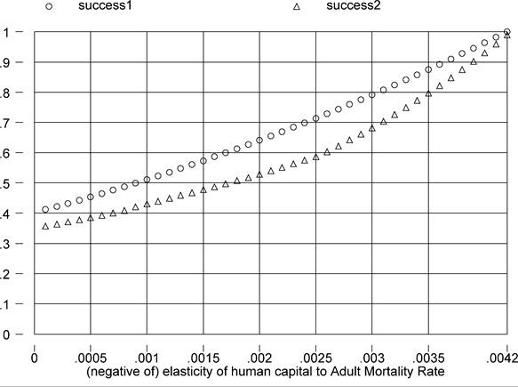
Figure 12. -φamr

and success.

Given his choices of functional form, however, this calibration implies that a one- percentage-point reduction in the probability of dying young is associated with a 1.68 percent increase in human capital, and hence in wages. Put another way, reducing the probability of dying before the age of 60 (as of age 15) by 6 percentage points has the same impact on wages as one extra year of schooling. This effect may seem a bit too large to be realistic. Given the somewhat tortuous - if ingenious - path through which Weil comes up with this calibration, I would tend to consider this number an upper bound.^[403]

One can perhaps improve on Weil’s exercise by exploiting as a proxy for health the information on average birthweight generated by Behrman and Rosenzweig (2004). The great advantage is that these authors also report estimates (based on within twin-pair re­gressions) of the economic returns to higher birthweight (as measured by wages). This should provide a more solid base for calibration. There are, however, several short­coming. First, birthweight may be less strongly correlated with health than the adult mortality rate. Second, the cross-section of mean birthweights refers to new borns in 1989, so it captures (a correlate of) the health of a cohort of workers that was not even in the labor force (aside from the most extreme cases of child labor) as of the date of our development accounting exercise (1996). Hence, one needs to assume a very high degree of persistence in cross-country differences in birthweights in order to put a lot of stock in this exercise. Third, the point estimate of the returns to birthweight are from a sample of US female twins, and one may question their applicability to the population at large.^[404]

With those caveats, Figure 13 plots the usual measures of success when we assume A_h = e^φbwB^iv, where BW is Behrman and Rosenzweig’s mean birthweight (in pounds), and φ_bw is the elasticity of human capital to birthweight. The number of countries is 83. Since birthweight is higher in rich countries a higher value of φ_bw increases the ex­planatory power of human capital. However, the value of φ_bw implied by Behrman and Rosenzweig’s log wage regressions is 0.076, which implies a trivially small improve­ment in the success of the factor-only model. This is substantively the same conclusion of Behrman and Rosenzweig, who report that the variance of φbwBW is less than one percent of the variance of log(y).

In sum, while the results with the adult mortality rate strongly imply that a correction for differences in health status is a first-order requirement in the measurement of human capital, those using birthweight are much less supportive. In light of the shortcomings of

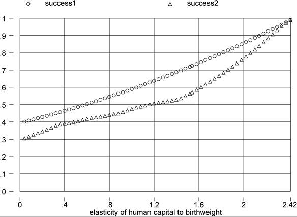
Figure 13. φb_w and success.

both exercises, however, it seems highly worthwhile to try and explore the matter further with more accurate indicators of health and more precisely calibrated parameters.

4.4. Social vs. private returns to schooling and health

Some additional important caveats about the nature of the calculations above is in order before I “set aside” human capital. Recall that the function φ(s) that we have used to map years of schooling into human capital was calibrated on estimates of private rates of return. Similarly, attempts at calibrating the health-human capital relation rely on observed private returns to health. But, as pointed out by various authors, and especially forcefully by Pritchett (2003), these private returns may bear little relationship to the social (or aggregate) return to education, which is of course what one would like to plug in our calculations.

As Pritchett points out, the social return to education may be higher or lower than the private one. Most growth theorists instinctively think about the former case, as they have in mind models with positive spillovers from human capital. However, Pritchett's review of the evidence is typical in finding very little empirical support for positive ex­ternalities.^[405] On the other hand, various versions of the education-as-signalling-device model, as well as models of rent seeking, imply that the social return to education is Iowerthanthe private return.^[406] This possibility is quite compelling. Note, however, that our calculations above imply that if we uniformly lower the social rate of return to ed­ucation, cross-country schooling inequality will explain even less of income inequality than it does in our benchmark calculation (see Figure 2).

38

Pritchett, however, also convincingly argues that the extent of rent seeking, and there­fore the extent to which the social return is below the private return, is much larger in poor countries. For example, in many poor countries the government employs an over­whelmingly large share of college graduates. This is sometimes the result of guaranteed- employment rules that commit the government to find employment to anyone with a tertiary degree. In contrast, in rich countries most college graduates work in the pri­vate sector. Since standard rent-seeking arguments imply that the government sector is intrinsically likely to make less efficient use of resources, this implies that on average the social return to education will be lower in poor countries. This effect is of course reinforced by the fact that poor countries are notoriously more prone to corruption and rent seeking than rich ones.

This will help. If the social rate of return to education (and health) is allowed to be higher in rich countries, then the variance of h will increase, and with it the explanatory power of the model. How important this could be quantitatively is hard to say, but by all means it would be worth finding out. A first exploratory step may be to break down the labor force into government-employees and private-sector workers. One may then retain the parameterization of the benchmark case for the private sector workers, but assume lower returns for government employees.

4.