The measure of our ignorance
The key empirical result that motivates this chapter is that in a simple framework with two factors of production, physical and human capital, a large fraction of the crosscountry income variance remains unexplained.
This result has been established by a variety of authors using a variety of techniques. Knight, Loayza and Villanueva (1993), Islam (1995), and Caselli, Esquivel and Lefort (1996), for example, used panel-datatechniques to estimate (1). They all found that, after controlling for factor accumulation, country-specific effects played a large role in output differences, and interpreted these fixed effects as picking up differences in efficiency. King and Levine (1994), Klenow and Rodriguez-Clare (1997), Prescott (1998), and Hall and Jones (1999), instead, used a calibration approach, and found that plausible parametrizations of (1) had limited explanatory power without large efficiency differences. These studies used cross-country national-account data on inputs and outputs, but Hendricks (2002) was able to reach similar conclusions by using earnings of migrants to the United States, and Aiyar and Dalgaard (2002) by using a dual approach involving factor prices rather than quantities. All these papers were inspired by - and written in response to - the challenge posed by the seminal contribution of Mankiw, Romer and Weil (1992).[376]
In this section I revisit the basic development-accounting finding. Because I want to set the stage for a variety of extensions of the basic model, I adopt the calibration approach, which offers more flexibility in experimenting with different parameter values and functional forms.[377]
I adopt as the benchmark Hall and Jones’ production function, according to which a country’s GDP, Y, is

where K is the aggregate capital stock and Lh is the “quality adjusted” workforce, namely the number of workers L multiplied by their average human capital h.
α is a constant. Clearly this is a special case of (1), where the residual A represents the efficiency with which factors are used. It is also clear that A corresponds to the standard notion of Total Factor Productivity (TFP), so until further notice I will speak of efficiency and TFP interchangeably.In per-worker terms the production function can be rewritten as

where k is the capital labor ratio (k = K/L). We want to know how much of the variation in y can be explained with variation in the observables, h and k, and how much is “residual” variation, i.e. must be attributed to differences in A. Clearly to answer this question we need, besides data on y, data on k and h, as well as a value for the capital share α.
2.1. Basicdata
The basic data set used in this chapter combines variables from two sources. The first is version 6.1 of the Penn World Tables [PWT61 - Heston, Summers and Aten (2002)], i.e. the latest incarnation of the celebrated Summers and Heston (1991) data set. From PWT61 I extract output, capital, and the number of workers. The second is Barro and Lee (2001), which I use for educational attainment. Several additional data sources will be brought to bear for specific exercises in later sections, but the data we construct here will be crucial to everything we do.
Previous authors have mostly used version 5.6 of the Penn World Tables (PWT56). They have therefore attempted to explain the world income distribution as of the late 1980s. By using version 6.11 am able to update the basic result to the mid-90s.
I measure y from PWT61 as real GDP per worker in international dollars (i.e. in PPP - this variable is called RGDPWOK in the original data set).[378]
I generate estimates of the capital stock, K, using the perpetual inventory equation
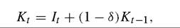
where It is investment and S is the depreciation rate.
I measure It from PWT61 as real aggregate investment in PPP.[379] Following standard practice, I compute the initial capital stock K0 as I0 /(g + S), where I0 is the value of the investment series in the first year it is available, and g is the average geometric growth rate for the investment series between the first year with available data and 1970. The rationale for this choice is tenuous: I/(g + S) is the expression for the capital stock in the steady state of the Solow model. We will see below whether results are very sensitive to this assumption, or for that matter to the others I am about to make, such as the one for S, which - following the literature -1 set to 0.06. To compute k, I divide K by the number of workers.[380]To construct human capital I take from Barro and Lee (2001) the average years of schooling in the population over 25 year old. Following Hall and Jones (1999) this is turned into a measure of h through the formula:
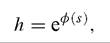
where is average years of schooling, and the function φ(s) is piecewise linear with slope 0.13 for ≤ 4, 0.10 for 4 < s ≤ 8, and 0.07 for 8 < s.7 The rationale for this functional form is as follows. Given our production function, perfect competition in factor and good markets implies that the wage of a worker with s years of education is proportional to his human capital. Since the wage-schooling relationship is widely thought to be log-linear, this calls for a log-linear relation between h and s as well, or something like h = exp(φss), with φs a constant. However, international data on education-wage profiles [Psacharopoulos (1994)] suggests that in Sub-Saharan Africa (which has the lowest levels of education) the return to one extra year of education is about 13.4 percent, the World average is 10.1 percent, and the OECD average is 6.8 percent.
Hall and Jones’s measure tries to reconcile the log-linearity at the country level with the concavity across countries.s is observed in the data every five years, most recently in 2000. Since s moves slowly over time, a quinquennial observation can plausibly be employed for nearby dates as well.
I treat a country as having “complete data” at date t if it has an uninterrupted investment series between 1960 and t, and it has an observation for s in 1995.8 With this definition, there are 94 countries with complete data in 1995, 94 in 1996, 91 in 1997, 90 in 1998, 87 in 1999, and 82 in 2000 (and 0 thereafter). Hence, I focus on 1996 as the most recent year that affords the largest sample. In this sample, for more than half of the countries the investment series starts in 1950.9
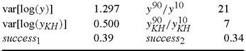
As is well known, per-capita income differences are enormous. The richest country in the sample (USA) has income per worker equal to 57,259 1996 international dollars, while the poorest (Zaire, today’s Democratic Republic of the Congo) has 630 - a ratio of 91. The ratio between the 90th (Canada) and the 10th percentile (Togo) of the income distribution, a measure of dispersion I’ll use prominently in the rest of the paper, is 21. The log-variance, another measure I’ll rely on heavily, is 1.30.
For the last ingredient required by Equation (3), α, I (implicitly) use US time-series data on the capital-share, whose long-run (and roughly constant) average value is 1/3. All these data choices will be subject to scrutiny in the rest of the chapter - indeed, this scrutiny is one of the chapter’s contributions.
2.2. Basic measures of success
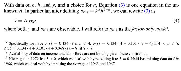
Throughout this chapter I will pursue the following version of the developmentaccounting question: how successful is the factor-only model at explaining crosscountry income differences? In other words, I will compare the (observed) variation in yHK to the (observed) variation in y.
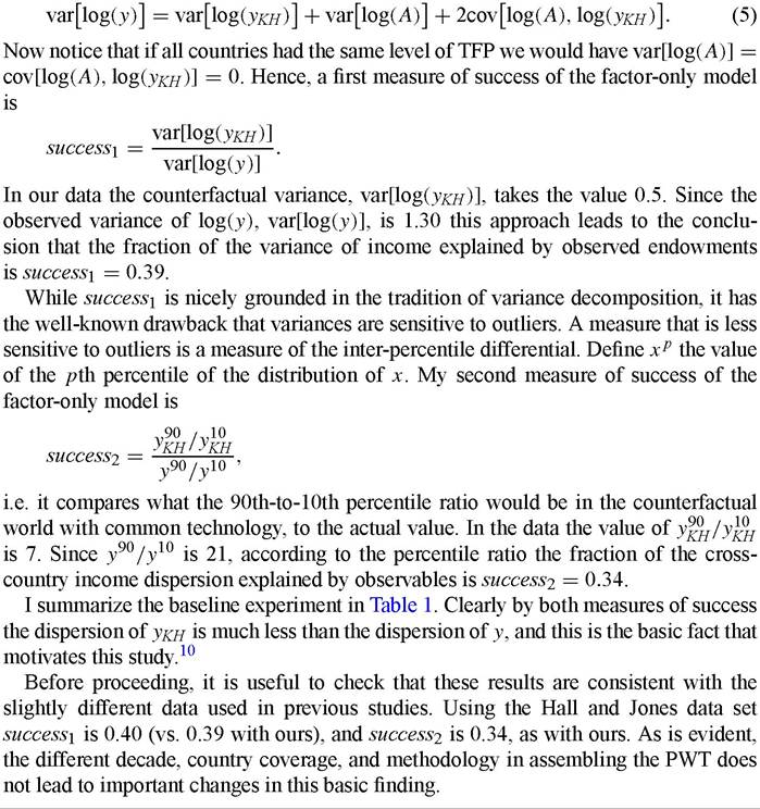
Clearly, this means that I am asking the following question. Suppose that all countries had the same level of efficiency A: what would the world income distribution look like in that case, compared to the actual one?To perform this assessment, I will look at two alternative measures. The first one is in the tradition of variance decompositions. From (4) we have
[1] Of course variation in yKH - even though much less than variation in y - is economically significant and interesting in its own right. For recent studies shedding light on the sources of variation in k and h see, e.g., Bils and Klenow (2000), Hsieh and Klenow (2003), and Gourinchas and Jeanne (2003).
Table 1
Baseline success of the factor-only model
2.3. Alternative measures used in the literature success1 essentially asks what would the dispersion of (log) per-capita income be if all countries had the same level of efficiency, A, and then compares this counter-factual dispersion to the observed one. Klenow and Rodriguez-Clare (1997) propose the alternative measure:
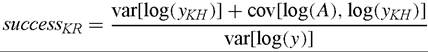
which differs from success1 for the covariance term in the numerator. In terms of Equation (5) successKR is equivalent to a variance decomposition in which the contribution from the covariance term is split evenly between A and yKH. Because in the data cov[log(A), log(yKH)] is positive (0.28) the Klenow and Rodriguez-Clare measure assigns a greater role to k and h than the simple ratio of variances: successKR is 0.60. Here I do not emphasize this measure because it does not answer the question: what would the dispersion of incomes be if all countries had the same A? As Klenow and Rodriguez-Clare explain, it asks the different question: “when we see 1% higher y, how much higher is our conditional expectation of yKH?” which in my opinion is not as intuitive.
Klenow and Rodriguez-Clare (1997) and Hall and Jones (1999) also work with a different version of the expression for per-capita income, because they rewrite (3) as
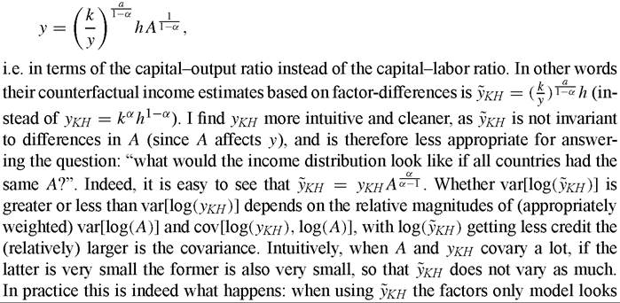
even more unsuccessful than when using yKH: success1 is as low as 0.22, and success2 is 0.20. Notice that relative to Klenow and Rodriguez-Clare (1997) we have made two methodological changes whose effects go in opposite directions: omitting the covariance term from success1 lowers the explanatory power of factors, while writing y in terms of the capital-labor ratio increases it. This is why we end up with results that are in the same ball park.
It is worth noting that Hall and Jones’ production function, Equation (2), is substantially more restrictive than the one used by some of the other authors in the literature. In particular Mankiw, Romer and Weil (1992) and Klenow and Rodriguez-Clare (1997) work with Y = KαHβLγ-α-β. Equation (2) is the special case where β = 1 - α. The great advantage of the Hall and Jones’ formulation is that it generates the log-linear relation between wages and years of schooling that we exploited to calibrate ½.11 Since wage data do seem to call for log-linear wage-education profiles, Hall and Jones’ restriction may be justified.
2.4. Sub-samples
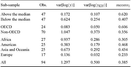
It may be interesting to take a look at the values that the success measures take in subsample of countries. This is done in Table 2, where I report success1 - as well as its two component parts - for the sub-samples of countries below and above the median per worker income; in and out of the OECD; and for the various continents. I also for convenience repeat the full-sample values. I do not report success2 because the small sample sizes make this variable hard to interpret.
Obviously the variation in log income per worker is smaller the smaller and more homogeneous the sub-samples. Perhaps more interestingly, it is also smaller in sub
Table 2
Success in sub-samples
11 With the Mankiw, Romer and Weil formulation the wage of a worker with 5 years of schooling is w(s^) = wL + WHh(s), where Wl is the wage paid to “raw” labor and wh is the wage per unit of human capital.
samples that tend to be richer on average (Above the median, OECD, Europe and Americas). It is indeed remarkable that, within the four continental groupings, the greatest variation in living standards is observed in Africa, a continent that is often depicted as flattened out by unmitigated and universal blight.
The success of the factor-only model is higher in the above the median and in the OECD samples than in the below the median and non-OECD samples, respectively. Hence, it is easier to explain income differences among the rich than among the poor. Furthermore, as indicated by comparison with the results for the full sample, it is easier to explain income differences among the rich than between the rich and the poor - while it is roughly as easy to explain within-poor differences as rich-poor differences. At the continental level, success is highest in the Americas, with roughly 50% of the log income variance explained, and lowest in Europe, with 23%. The latter result is entirely driven by the inclusion of the lone eastern European country (Romania), whose very high level of human capital makes it difficult to explain its very low income [Caselli and Tenreyro (2004) generalize this finding to a broader sample]. When Romania is excluded the success of the factor-only model for Europe is virtually perfect. In sum, the factor-only model works the worst where we need it most: i.e. when poor countries are involved.[381]
3.