Other symptoms of a GPT
So far we have provided some measures of the three qualities of a GPT - its pervasiveness, its rate of improvement, and its innovation-spawning tendency. Now we turn to less direct measures as suggested by various theoretical models that deal with GPTs.
These models predict the following symptoms:1. Productivity should slow down - The new technology may not be user-friendly at first, and output may fall for a while as the economy adjusts.
2. The skill premium should rise - If the GPT is not user-friendly at first, skilled people will be in greater demand when the new technology arrives and their earnings should rise compared to those of the unskilled.
3. Entry, exit and mergers should rise - These are alternative modes for the reallocation of assets.
4. Stock prices should initially fall - The value of old capital should fall. How fast it falls depends on the way that the market learns of the GPT’s arrival.
5. Young and small firms should do better - The ideas and products associated with the GPT will often be brought to market by new firms. The market share and market value of young firms should therefore rise relative to old firms.
6. Interest rates and the trade deficit - The rise in desired consumption relative to output should cause interest rates to rise or the trade balance to worsen.
These, roughly speaking, are the hypotheses that emerge from the theoretical work on GPTs. Now we examine each empirically in turn, and as we go through the facts, we shall mention some of the relevant theories.
3.1. Productivity slowdown
As Bahk and Gort (1993) show, even in routine activities, learning seems to cause delays of several years before plant productivity peaks. It is far from settled, however, whether IT is the reason for the productivity slowdown - Bessen (2002) finds that IT did cause a big part of the slowdown, whereas Comin (2002) argues the opposite.
It is also not yet definitely known from the work of Caballero and Hammour (1994) and others whether recessions at business-cycle frequencies are episodes of heightened reallocation. At any rate, the theoretical models of Atkeson and Kehoe (1993), Hornstein and Krusell (1996), Jovanovic and Nyarko (1996), Greenwood and Yorukoglu (1997) and Jovanovic and Rousseau (2002a) emphasize various adjustment costs and learning delays that may cause output to fall at first when a GPT arrives. David (1991) argues that the speed with which a new technology diffuses depends on the pool of investment opportunities that are available when it arrives, and remarks that the quality of this pool in the late 1960s was low because a large backlog from the post-war period had just and finally been eliminated. He also points out that there can often be “slippage” between the technological frontier and implementation due to high input costs and the slow introduction of complementary products.Figure 1 shows that productivity did not rise quickly in the early phases of the two GPTs, though there is some evidence of greater productivity between 1918 and 1929 and after 1997 or so. Productivity was high in the early years of the Electrification period but fell rapidly as the technology matured. It stayed low through the Depression and 1940s, and then rose rapidly before the IT-age arrived. This pattern is consistent with David’s view of exhausted investment opportunities. And while it is interesting to consider the productivity slowdown after 1971, it is also important to recognize that productivity is considerably higher today than it was before IT’s arrival.
3.2. The skill premium
As Nelson and Phelps (1966) and Griliches (1969) argued, and Bartel and Lichtenberg (1987) and Krusell et al. (2000) have confirmed, new technology should raise the relative earnings of the skilled. Figure 18 presents a series for the earnings of skilled relative to unskilled labor. We construct the series by combining estimates of the wage ratio for urban skilled and unskilled workers for 1870-1894 from Williamson and Lindert (1980, p.
307) with estimates of the ratio of clerical to manufacturing production wages for 1895-1938 and the returns to 16 versus 12 years of schooling for men for 1939-1995 from Goldin and Katz (1999b).[132]Although interpreting time series patterns in a continuous series formed from such disparate sources must be done with caution, we note that the series does have a U-shape, with the skill premium high in the early stages of Electrification (i.e., 1890 to 1918) and then rising rapidly during the post-1978 part of the IT epoch. We suspect that the decline in the skill premium from 1918-1924 would have been less deep, and thus the overall U-shape of Figure 18 more apparent, had it not been for the rapid rise of the public higher-education system after the end of World War I [see Goldin and Katz (1999a,p. 10)].
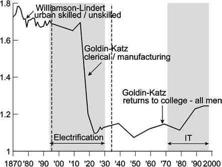
Figure 18. Theskillpremium.
3.3. Entry, exit, and mergers should rise
Gort (1969) argued that technological change will generate merger waves. Evidence since then has shown that mergers and takeovers play a re-allocative role for an economy’s stock of human and physical capital. Lichtenberg and Siegel (1987), McGuckin and Ngyen (1995) and Schoar (2002) find that the productivity of a target firm rises following a takeover. Jovanovic and Rousseau (2002b, 2002c) study the trade-off between exits and acquisitions at the margin for an economy that needs to update its capital stock. This last pair of papers shows that, at times when the value of organization capital is high, firms are more likely to place themselves on the merger market than to disassemble and sell their assets. Further, reallocation of assets among firms in general (i.e., by merger, consolidation, or purchases of unbundled used capital) is more likely to occur than purchases of new capital when firms need to make large adjustments to their capital stocks because of fixed costs associated with entering the merger market.
We believe that both of these conditions are likely to hold during times of sweeping technological change.The U-shaped top line of Figure 19 is our estimate of the total amount of capital that has been reallocated on the U.S. stock market from 1890 to 2003. Its components are the stock market capitalization of entering and exiting firms divided by two, and the value of merger targets.[133] Entries and exits divided by two, given by the center line, is a rough measure of how much capital exits from the stock market and comes back in under different ownership, or at least under a different name.[134] The lower line is the stock-market value of merger targets. Regardless of whether reallocation occurs through mergers or through entry and exit, it is much more prevalent during the periods that we associate with Electrification and IT.
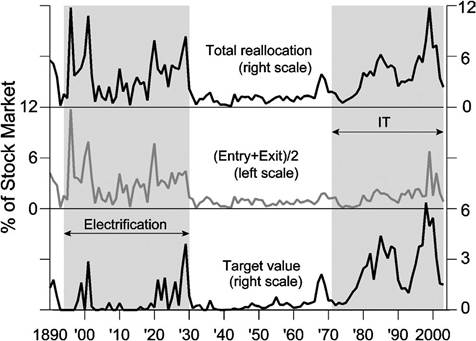
Figure 19. Reallocated capital and its components as percentages of stock market value, 1890-2003.
3.4. Stock prices should fall
The value of old capital should fall suddenly if the arrival of the GPT is a surprise, as in Greenwood and Jovanovic (1999), Hobijn and Jovanovic (2001), Jovanovic and Rousseau (2002a) and Laitner and Stolyarov (2003), or more gradually as in Helpman and Trajtenberg (1998a, 1998b). Figure 20 shows that the stock market declined in 1973-1974.[135] No such sudden drop is visible for stock prices in the early 1890s. Why not? Maybe because the market was thin and unrepresentative in those days, with railway stocks absorbing a large share of market capitalization. More likely, the realization that the new technology would work well was more gradual and not prompted by any single event such as the activation of the Pearl Street power station in 1882 or the completion of the Niagara Falls dam in 1894.
In other words, perhaps a decline in the stock market did not occur early in the Electrification period because the events of the early 1890s were foreseen, as would be the case in Helpman and Trajtenberg (1998a, 1998b).
It also could be, as in Boldrin and Levine (2001), that old capital is essential to the production of new capital and that its value may not fall in quite the way that it would when capital can be produced from consumption goods alone, as is the case in many growth models including Jovanovic and Rousseau (2002a).If stock price declines were caused by the threat of IT to incumbents, this should relate especially to those sectors that later invested heavily in IT. Hobijn and Jovanovic (2001, p. 1218) confirm this using regression analysis.
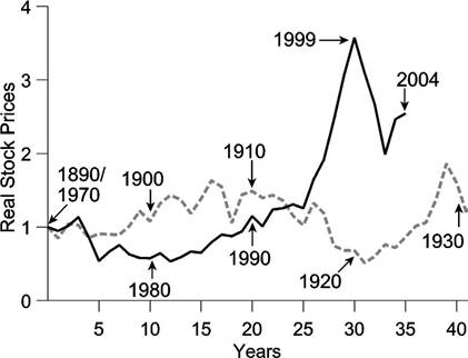
Figure 20. The real Cowles/S&P stock price index across the two GPT eras.
3.5. Young firms should do better
If new technologies are brought to market most effectively by new firms, we would expect younger firms in general to perform better than older firms during the eras of GPT adoption. The evidence on this hypothesis turns out to be mixed, but positive overall.
3.5.1. The age of the leadership
As a GPT takes hold, we should not only expect to see firms coming to market more quickly, but the market leaders getting younger as well. In other words, every stage in the lifetime of the firm should be shorter. This stands in contrast to Hopenhayn (1992), in which the age distribution of an industry’s leadership is invariant when an industry is in a long-run stochastic equilibrium. That is, the average age of, say, the top 5 percent or top 10 percent of firms is fixed. Some leaders hold on to their positions and this tends to make the leading group older, but others are replaced by younger firms, and this has the opposite effect. In equilibrium the two forces offset one another and the age of the leadership stays the same. Keeping the age of the leaders flat requires, in other words, constant replacement.
Figures 21 and 22 plot the value-weighted average age of the largest firms whose market values sum to 5 and 10 percent of GDP, respectively.
A firm’s “age” is measured as the number of years since incorporation and since being listed on a major stock exchange. We label some important entries and exits from this group in Figure 21 (with exits denoted by “X”). The two figures show that, overall, the age of the leaders is anything but flat. It sometimes rises faster than the 45o line, indicating that the age of the leaders is rising faster than the passage of time. At other times it is flat or falling, indicating replacement.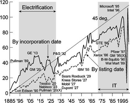
Figure 21. Average age (in years) of the largest firms whose market values sum to 5 percent of GDP, 1885-2001.
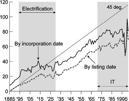
Figure 22. Average age (in years) of the largest firms whose market values sum to 10 percent of GDP, 1885-2001.
Based upon years from incorporation, for example, the leading firms were being replaced by older firms over the first 30 years of our sample, because the solid line is then steeper than the 45o line. In the two decades after the Great Depression the leaders held their relative positions as the 45o slopes of the average age lines show. The leaders got younger in the 1990s, and their average ages now lie well below the 45o line.[136] Both figures show, however, that the lines are flat or falling during the Electricity and IT periods, so that replacement at these times was high. This is best seen in Figure 22.
3.5.2. The age of firms at their IPO
According to the third “innovation-spawning” characteristic, when a GPT arrives it gives rise to new projects that are unusually profitable. When such projects arrive, firms will be more impatient to implement them. When it is new firms that come upon such projects (rather than incumbents), they will feel the pressure to list sooner. This argument is developed and tested in Jovanovic and Rousseau (2001). We argue there that the Electricity- and IT-era firms entered the stock market sooner because the technologies that they brought in were too productive to be kept out of the market for very long.
Figure 23 shows HP-filtered average waiting times from founding, first product or process innovation, and incorporation to exchange listing based upon individual company histories and our backward extension of the CRSP database.21 The vertical distance between the solid and dotted lines shows that firms often have their first innovation soon after founding, but that it then takes years, even decades, to list on a stock ex- change.22 We interpret this delay as a period during which the firm and possibly its lenders learn about what the firm’s optimal investment should be. But when the technology is highly innovative, the incentive to wait is reduced and the firm lists earlier, which is what the evidence shows.
Table 4 lists the first product or process innovation for some of the better-known companies, along with their dates of founding, incorporation, and stock exchange listing. It also includes the share of total market capitalization that can be attributed to each firm’s common stock at the end of 2003. The firms appearing in the table separate into roughly 3 groups: those based upon electricity and internal combustion, those based upon chemicals and pharmaceuticals, and those based upon the computer and Internet. Let us consider a few of the entries more closely:
comes from Microsoft’s enormous price appreciation in 1999, when it was worth more than 5 percent of GDP on its own, and its rapid decline in 2000, which transferred the full 5 percent share to GE. The two firms split the 5 percent share in 2001.
21 Listing years after 1925 are those for which firms enter CRSP. For 1890-1924, they are years in which prices first appear in the NYSE listings of The Annalist, Bradstreet’s, The Commercial and Financial Chronicle or The New York Times. The 6,632 incorporation dates used to construct Figure 23 are from Moody’s Industrial Manual [Moody’s Investors Service (1920, 1928, 1955, 1980)], Standard and Poor’s StockMarket Encyclopedia [Standard and Poor’s Corporation (1981, 1988, 2000)] and various editions of Standard and Poor’s StockReports [Standard and Poor’s Corporation (1971-2003)]. The 4,221 foundings are from Dun and Bradstreet’s Million Dollar Directory [Dun and Bradstreet, Inc. (2003)], Moody’s, Kelley (1954), and individual company web sites. The 482 first innovations were obtained by reading company histories in Hoover’s Online [Hoover’s, Inc. (2000)] and company web sites. We linearly interpolate the series between missing points before applying the HP-filter to get the time series in Figure 23.
22 Figure 23 includes several years in the 1970s and early 1980s for which it appears that the average time from first innovation to listing exceeds that from founding to listing. This is a result of differences in the sample sizes used to construct each line.
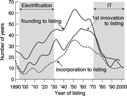
Figure 23. Waiting times to exchange listing, 1890-2003.
• Electricity/Internal Combustion Engine - Two of largest companies in the United States today are General Electric (GE) and AT&T. Founded in 1878, GE accounted for 2.1 percent of total stock market value at the end of 2003, and had already established a share of over 2 percent by 1910. AT&T, founded in 1885, contributed 4.6 percent to total market value by 1928, and more than 8.5 percent at the time of its forced breakup in 1984. Both were early entrants of the Electricity era. GE’s founding was based upon the invention of the incandescent light bulb in 1879, while AT&T established a long-distance telephone line from New York to Chicago in 1892 to make use of Bell’s 1876 invention of the telephone. Both technologies represented quantum leaps in the modernization of industry and communications, and both firms brought these technologies to the NYSE about 15 years after founding. General Motors (GM) was an early entrant to the automobile industry, listing on the NYSE in 1917 - nine years after its founding. By 1931 it accounted for more than 4 percent of stock market value, and its share would hover between 4 and 6.5 percent until 1965, when it began to decline gradually to its share in 2003 of only 0.2 percent. These examples suggest that many of the leading entrants at the turn of the 20th century created lasting market value. Further, the ideas that sparked their emergence were brought to market relatively quickly.
• ChemicalsPharmaceuticals - Procter and Gamble (P&G), Bristol-Myers Squibb and Pfizer are both leaders in their respective industries, but took much longer to list on the NYSE than the Electrification-era firms. In fact, P&G and Pfizer were established before 1850, and thus predate all of them. Despite P&G’s early start and the creation of the Ivory soap brand in 1879, it was not until 1932 that the company took its place among the largest U.S. firms by exploiting advances in radio transmission to sponsor the first “soap opera”. Pfizer’s defining moment came when it developed a process for mass-producing the breakthrough drug penicillin
Table 4
Key dates in selected company histories
| Company name | Founding date | 1st major product or process innovation | Incorporation date | Listing date | % of stock market in 2003 |
| General Electric | 1878 | 1880 | 1892 | 1892 | 2.09 |
| AT&T | 1885 | 1892 | 1885 | 1901 | 0.11 |
| Detroit Edison | 1886 | 1904 | 1903 | 1909 | 0.04 |
| General Motors | 1908 | 1912 | 1908 | 1917 | 0.20 |
| Coca Cola | 1886 | 1893 | 1919 | 1919 | 0.83 |
| Pacific Gas & Electic | 1879 | 1879 | 1905 | 1919 | 0.08 |
| Burroughs/Unisys | 1886 | 1886 | 1886 | 1924 | 0.03 |
| Caterpillar | 1869 | 1904 | 1925 | 1929 | 0.19 |
| Kimberly-Clark | 1872 | 1914 | 1880 | 1929 | 0.20 |
| Procter & Gamble | 1837 | 1879 | 1890 | 1929 | 0.87 |
| Bristol-Myers Squibb | 1887 | 1903 | 1887 | 1933 | 0.37 |
| Boeing | 1916 | 1917 | 1916 | 1934 | 0.23 |
| Pfizer | 1849 | 1944 | 1900 | 1944 | 1.81 |
| Merck | 1891 | 1944 | 1934 | 1946 | 0.69 |
| Disney | 1923 | 1929 | 1940 | 1957 | 0.32 |
| Hewlett-Packard | 1938 | 1938 | 1947 | 1961 | 0.47 |
| McDonalds | 1948 | 1955 | 1965 | 1966 | 0.21 |
| Intel | 1968 | 1971 | 1969 | 1972 | 1.40 |
| Microsoft | 1975 | bgcolor=white>19801981 | 1986 | 1.99 | |
| America Online | 1985 | 1988 | 1985 | 1992 | 0.52 |
| Amazon | 1994 | 1995 | 1994 | 1997 | 0.14 |
| E-Bay | 1995 | 1995 | 1996 | 1998 | 0.28 |
Source: Data from Hoover's Online, Kelley (1954), and company web sites.
Note. The first major products or innovations for the firms listed in the table are: GE 1880, Edison patents incandescent light bulb; AT&T 1892, completes phone line from New York to Chicago; DTE 1904, increases Detroit’s electric capacity six-fold with new facilities; GM 1912, electric self-starter; Coca Cola 1893, patents soft-drink formula; PG&E 1879, first electric utility; Burroughs/Unisys 1886, first adding machine; CAT 1904, gas driven tractor; Kimberly-Clark 1914, celu-cotton, a cotton substitute used in WWI; P&G 1879, Ivory soap; Bristol-Myers Squibb 1903, Sal Hepatica, a laxative mineral salt; Boeing 1917, designs Model C seaplane; Pfizer 1944, deep tank fermentation to mass produce penicillin; Merck 1944, cortisone (first steroid); Disney 1929, cartoon with soundtrack; HP 1938, audio oscillator; McDonalds 1955, fast food franchising begins; Intel 1971, 4004 microprocessor (8088 microprocessor in 1978); Microsoft 1980, develops DOS; AOL 1988, “PC-Link”; Amazon 1995, first online bookstore; E-Bay 1995, first online auction house.
during World War II, and the good reputation that the firm earned at that time later helped it to become the main producer of the Salk and Sabin polio vaccines. In Pfizer’s case, like that of P&G, the company’s management and culture had been in place for some time when a new technology (in Pfizer’s case antibiotics) presented a great opportunity.
• Computer/IT - Firms at the core of the recent IT revolution, such as Intel, Microsoft and Amazon, came to market shortly after founding. Intel listed in 1972, only four years after starting up, and accounted for 1.4 percent of total stock market value at the end of 2003. Microsoft took eleven years to go public. Conceived in an Albuquerque hotel room by Bill Gates in 1975, the company, with its new disk operating system (MS-DOS), was perhaps ahead of its time, but later joined the ranks of today’s corporate giants with the proliferation of the PC. In 1998, Microsoft accounted for more than 2.5 percent of the stock market, but this share fell to 1.5 percent over the next two years in the midst of antitrust action. By the end of 2003 its share had recovered somewhat to nearly 2 percent of the stock market. Amazon caught the Internet wave from the outset to become the world’s first online bookstore, going public in 1997 - only three years after its founding. As the complexities of integrating goods distribution with an Internet front-end came into sharper focus over the ensuing years, however, and as competition among Internet retailers continued to grow, Amazon’s market capitalization by 2003 had fallen to 0.14 percent of total stock market value.
These firms, as well as the others listed in Table 4, are ones that brought new technologies into the stock market and accounted for more than 13 percent of its value at the close of 2003. The firms themselves also seem to have entered the stock market sooner during the Electricity and IT eras, at opposite ends of the 20th century, than firms based on mid-century technologies.
When firms gather less information before investing, the investments that they undertake will be riskier. One may conjecture that if new entrants waited less before investing during the GPT eras, then incumbents also undertook projects earlier than they would have normally. In these cases, the resulting investments would be riskier than if more time were allowed to plan them. Moreover, the newness of the GPT would add further risk. On all these grounds, we would expect interest rate differentials on the average investment to be higher in the GPT eras.
Figure 24, which shows the spread between interest rates on riskier and safe investments since 1885, shows that this hasbeenforthe most part the case.[137] Itis important to note that we formed the series in Figure 24 by joining three different spreads together, and that the “safe” asset is a long-term U.S. government bond before 1920 and a shortterm U.S. Treasury bill thereafter, yet the fluctuations in this series should still reflect risk perceptions reasonably well, at least to the extent that term premia rather than riskiness are the main factors that lead to yield differentials among the various government securities.
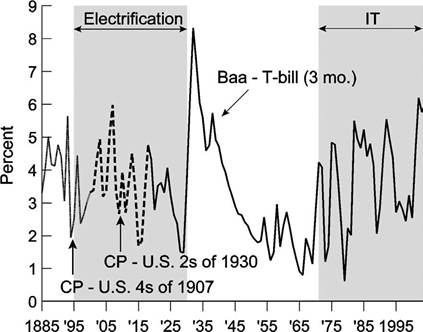
Figure 24. Nominal interest rate spreads between riskier and safer bonds, 1885-2003.
Duringthe Electrification period, spreads rose between 1894 and 1907, which is when uncertainty about the usefulness and possibilities for adoption of the new technology was greatest. Spreads fell after that as the future of Electricity became clearer. In the IT era, spreads have a generally-upward trend throughout, though they did fall for a while in the late 1990s. This may well reflect the lag in the widespread adoption of IT. The spread’s sharp rise in 1930 and very slow decline over the next 15 years probably has to do with the macroeconomic instability induced by events prior to and during the Great Depression, and then the heavy borrowing by the U.S. government to finance World War II, which raised rates on T-bills.
Another measure of risk perceptions can be obtained from the distribution of ratings for issues of new corporate bonds. Figure 25 uses data from Hickman (1958, pp. 153-154) and Atkinson (1967, p. 97) for the period from 1908-1965 to show four- year averages, starting at the dates shown on the horizontal axis, of the percent of the total par value of rated new corporate bond issues that received a Moody’s rating of single-A or lower and Ba or lower. In other words, the solid line excludes the highest rated bonds (i.e., classes Aaa and Aa), but includes some investment grade bonds (i.e., A and Baa) along with the sub-investment grades (i.e., Ba and lower). The dashed line includes only the sub-investment grades.
The dashed line in Figure 25 indicates that subinvestment grade bonds made up a larger part of the value of total rated new issues during the Electrification era than after the start of the Great Depression, and though these data end in 1965, we note that subinvestment grade issues began to rise again only on the eve of the IT revolution in the mid-1960s. The solid line shows that issues of bonds not receiving the highest Moody’s ratings actually rose during the latter part of the Electrification era, peaking in the 1924-1927 period, which was when a host of Electricity-related innovations and appliances were being brought to market. This does not imply an increase in junk-bond
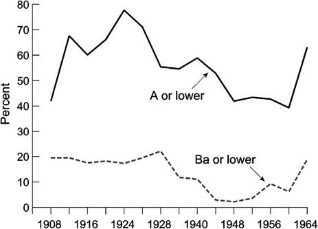
Figure 25. Percent of rated corporate bond offerings with Moody’s ratings of A or lower and Ba or lower, four-year averages, 1908-1965.
issuance at this time, but rather is consistent with the view that investors recognized the risks involved with large-scale use of the new technology and were a bit more cautious about overpaying for debt securities associated with it.
3.5.3. The stock market performance of the young vs. old after entry
Young firms are smaller. If “creative destruction” does indeed mean that old firms give way to young firms, then we should see signs of it in Figure 26, which depicts the relative appreciation of the total market value of small versus large firms since 1885.[138] We define “small” firms as those in the lower quintile of CRSP, and “large” firms as those in the upper quintile. The regression line in Figure 26 (with t-statistics in parentheses) shows small firms outperforming large ones in the long run and an annual growth premium of about 7.5 percent. But the two GPT eras do not show a faster rise in relative appreciations than other times, and this is puzzling. Surprisingly, recessions do not seem to hurt the long-term prospects of small firms: The relative index rises in 10 of the 23 NBER recessions.
The two periods that we wish to focus on are 1929-1931 and the early 1970s. In both periods, the small-capitalization firms lost out relative to the large-capitalization ones. The first period comes at the end of the Electrification era and the relative decline of smaller firms is what one would have expected. But the early 1970s come at the beginning of a new GPT, and small firms should have outperformed the large firms at
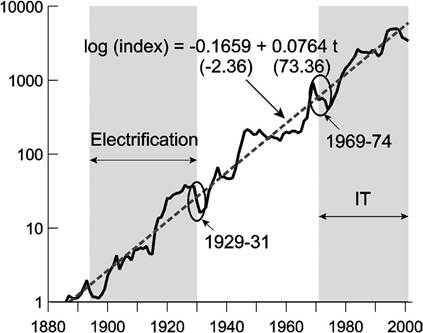
Figure 26. The relative capital appreciations of small vs. large firms, 1885-2001.
that time. Yet the opposite happened. It is only after 1974 that the small-capitalization firms start to perform better.
Regression evidence on age and stock market performance. If the GPT is brought in by young firms, then the capital loss imposed by the GPT’s arrival should fall more heavily on old firms. To test this using data on individual firms, let
Ai = age since listing of firm i in 1970;
Si = share (in firm i’s sector) of IT capital in the capital stock in 2001.
This measures a firm’s exposure to the impact of the new technology within its sector. We use the change in a firm’s stock price over intervals that start in 1971 and end in 1975,1980,1985,1990 and 1995 as measures of expected performance. These should reflect the market’s assessment of how well the firm will handle the consequences of the GPT. The regressions take the form

We summarize the firm-level results in Table 5.
The interaction between the firm’s age (A) and its exposure to the new technology (S) is negative and significant only when the period during which we measure price appreciation extends to 1990 and 1995. We would have expected this coefficient to be negative always, since older firms in sectors where IT would become important would be less able to adjust to the new technology than newer firms. The interaction term has a positive coefficient for the 1971-1975, 1971-1980 and 1971-1985 periods, but it is
Table 5
Age and stock market performance
Dependent variable: ln(Pt +i/Pt)
| 1971-1975 | 1971-1980 | 1971-1985 | 1971-1990 | 1971-1995 | |
| constant | -0.737 | -0.143 | 0.152 | -0.057 | 0.577 |
| (-24.3) | (-2.96) | (2.58) | (-0.59) | (6.06) | |
| A | 0.007 | -0.001 | -0.001 | 0.003 | -0.002 |
| (6.40) | (-0.46) | (-0.55) | (0.97) | (-0.51) | |
| S | -3.497 | -2.266 | -1.035 | -0.602 | 2.719 |
| (-7.60) | (-3.37) | (-1.20) | (-0.46) | (1.88) | |
| A * S | 0.047 | 0.043 | -0.016 | -0.122 | -0.106 |
| (2.22) | (1.14) | (-0.39) | (-2.09) | (-1.76) | |
| R2 | 0.089 | 0.009 | 0.003 | 0.006 | 0.012 |
| N | 2218 | 1814 | 1367 | 981 | 843 |
Note. The table presents coefficient estimates for the subperiods included in the column headings with t-statistics in parentheses. The R2 and number of observations (N) for each regression appear in the final two rows.
statistically Significantonly for the 1971-1975 period. Itthus seems that IT firms took a long time to realize gains in the market after the technology’s arrival. There are not very many firms with continuous price data prior to 1900, but we have enough observations to attempt the same regression for the Electrification era. In this case, we got
with t-statistics in parentheses and R2 = 0.015, N = 56. In this very small sample, we do not see a direct effect of age on capital depreciation as Electrification got underway, and the interaction term is not statistically significant.
3.6. Consumption, interest rates, and the trade deficit
If it is unanticipated, the arrival of a GPT is good news for the consumer because it brings about an increase in wealth. How quickly wealth is perceived to rise depends on how quickly the public realizes the GPT’s potential for raising output. The rise in wealth would raise desired consumption. But to implement the GPT firms would also need to increase their investment. Therefore aggregate demand would rise, and in a small open economy this would lead to a trade deficit. In a closed economy, on the other hand, since income does not immediately rise, the rise in aggregate demand would cause the rate of interest to rise so that the rise in aggregate demand would be postponed.
How much consumption rises depends on two factors. The first is the GPT’s pervasiveness worldwide - if the entire world is equally affected then consumption could not
rise right away and the main effects would be transmitted though the rate of interest. The second is the openness of the U.S. economy. Even if, say, the United States were the only country affected by the GPT, the rise in consumption would be related to how easily capital could flow in.
In these respects, the IT episode differs from the Electrification episode in several important respects. Capital inflows into the United States simply were not in the cards during a large part of the Electrification episode. World War I exhausted the European nations and the United States could not borrow from the rest of the world to finance its electrification-led expansion - it was instead a creditor during this period. Moreover, even if the war had not taken place, it is not clear whether the United States could have borrowed much from the rest of the world because Britain, Germany, France, and several other countries were undergoing the same process - Electrification was more synchronized across the developed world than IT has so far been.
In sum, we would expect the United States to have behaved more like a closed economy during the Electrification era and more like a small open economy during the IT era. Specifically, we would expect to see
(1) a larger rise in the trade deficit during the IT era than during the Electrification era,
(2) a smaller rise in consumption during the Electrification era then during the IT era,
(3) a larger rise in the rate of interest during the Electrification era.
3.6.1. Thetradedeficit
Figure 27, which plots the trade deficit as a percentage of GNP since 1790 along with an HP trend, shows sharply-rising trade deficits at the start of the IT revolution, though not in the early years of Electrification.[139] The trade deficit indeed opens up fairly dramatically during the IT era, whereas during the Electrification era we see a surplus. As we mentioned, this surplus was driven by the various Colonial wars that took place at the turn of the century and, of course, by World War I.
3.6.2. The consumption-income ratio
We expected to see a smaller rise in consumption during the Electrification era than during the IT era, and after we adjust for the downward long-run trend, this is indeed what has happened. Private consumption rises gradually during each GPT era, and this is set against a long-run secular trend for private consumption that is negative. Figure 28 shows the ratio of consumption to GDP since 1790.[140] As our GPT hypotheses would
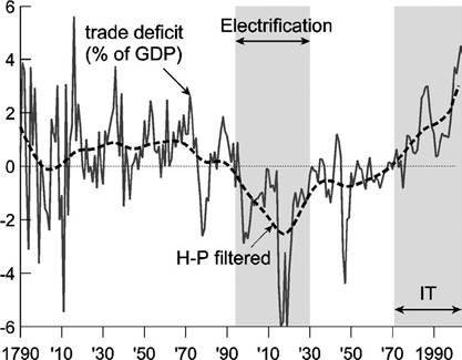
Figure 27. The trade deficit as a percent of GDP, 1790-2003.
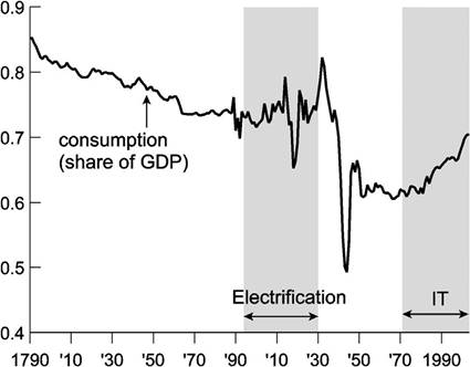
Figure 28. The ratio of consumption to income, 1790-2003.
suggest, the arrival of Electricity in 1890 seems to mark the end of a long-term decline in the ratio that been underway for a century. And though the level of the series falls during the Great Depression and World War II, never to return to its pre-1930 levels, consumption takes another sharp upward turn near the start of the IT revolution and continues to rise.
table 9, pp. 25-26) for 1790-1889. The BEA figures are for personal consumption, but the Kendrick and Berry figures include the government sector as well. Since consumption in the government sector was much smaller prior to World War I, we suspect that the downward trend in the 19th century is a result of changing private consumption patterns rather than a reduction in the government sector’s consumption.
3.6.3. Interest rates
We expected a larger rise in the rate of interest during the Electrification era than during the IT era. Relative to HP trends, the evidence is not favorable. Figure 29 shows that ex-post real interest rates were about the same during the two GPT eras, and much lower in the middle 40 unshaded years of the 20th century.[141] The dashed line is the HP detrended series. The averages are presented in Table 6. We note that the ex-post rate is quite high in the first era, before 1894. If the arrival of electricity and its impact was foreseen prior to 1894, interest rates would have risen earlier, but this probably does not explain why they were so high then. More likely, the pre-1894 era reflects a lack of financial development: The stock market was small then, and the financial market not as deep. This may have given rise to an overall negative trend in interest rates over the 134-year period as a whole.
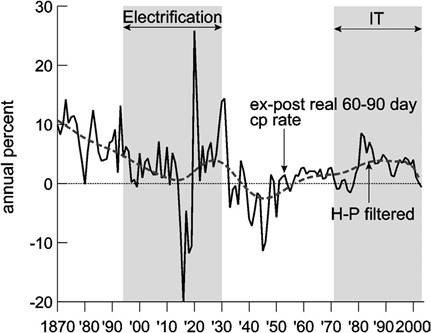
Figure 29. The ex-post real interest rate on commercial paper, 1870-2003.
Table 6
| Era | Ex-post real interest rate |
| 1870-1893 1894-1930 1931-1970 1971-2003 | 7.78 2.61 -0.16 2.75 |
4.