The Demand Law as Solved by Hildenbrand (1994)
For simplicity, we suppose a one-commodity world, as proposed by Lewbel (1994). In his exposition, an essential feature of Hildenbrand’s solution is condensed, so we do not take into account relative prices.
We saw in the Pareto-Slutsky equation of a one-commodity world that a supplemented item with income compensated to keep the same satisfaction is canceled out by the income effect: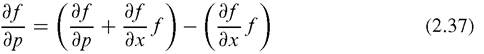
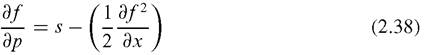
However, a trivial transformation of this equation, replacing the first item with s (the substitution effect), leads to:
2.2.4.1 A Sufficient Condition of the Demand Law in Hildenbrand (1994)
We introduce a population of heterogeneous consumers, so we have a distribution of individual demands {f1,..., f∙,..., fn} constituted by individuals i = 1,..., n. We omit the index i for a while. We also define a new function R(x):
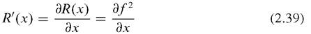
It is clear from the above that:

If we apply operator E to a demand distribution, we will obtain a new formulation of the Pareto-Slutsky equation:
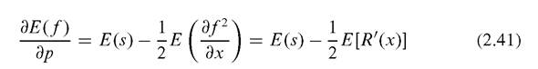
It follows from the property of the substitution effect that:
Hence our new function R(x) can be written: 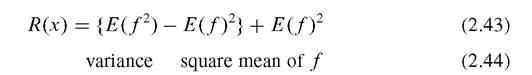
We can therefore measure the spread of demand by R(x). Demand, as well as heterogeneity of households, is greater as R(x) increases.
Suppose that p is a density function of income x. It then holds that:
It is therefore always certain, because of the property of R(x), that x increases.

Again, this is the demand law. It is verified by a sufficient condition that the spread of demand R(x) is greater as income x increases.
2.2.4.2 The Significance of Hildenbrand’s Finding
In traditional economics, price fluctuations overwhelmingly dominate changes in household demand almost everywhere. The demand law is distorted by the income effect. We have already shown that the direction of household demand is never driven only by price changes. Because of Hildenbrand’s (1994) contribution, we also know that class structure works to create a normal form of the demand law. It is quite interesting that a seemingly ‘normal’ law can actually be realized by supplementing a social factor: the existence of heterogeneous agents.
This perspective may be diagrammatically depicted (see Fig. 2.7). First, we recognized that income effects are not auxiliary, even where price-sensitive behavior is dominant, as long as prices appear independent, hence there are different forces: prices, demand and income classes. We can then show the real facets of interacting prices and demands with different income classes. As Fig. 2.7 shows, we need a multi-dimensional view. Our vision depends on which facet we view. The observation of consumer demand should not be limited to a particular facet where price-sensitive behavior could be dominant if prices are largely independent.
2.3