The Discrete Choice Model of Different Modes
Before we proceed to discuss the demand law itself, I turn to an alternative choice model or utility formulation, leaving the individual stage. Concentrating on intrinsic preference ignores the construction of chosen preferences in a group.
Without knowing about the whole of society, we cannot predict the market demand as a whole. It would be very difficult to attain a macroscopic view of demand simply by aggregating individual rationality. An alternative model was therefore proposed by Luce (1959), and is often called the multinomial logit model. It has been widely applied to practical estimation in many industries. Daniel Little McFadden, who was working on this model, was awarded a Nobel Prize in 2000, marking the fact that this is now considered an important economic model. See McFadden (1984).[27]In Luce’s original model (Luce 1959), there is a finite number of alternatives that can be explicitly listed. Suppose that there is the universal choice set U. The subset of this that is considered by a particular individual is called the reduced choice set C. A subset of C is denoted by S.It then holds: S c C c U.Ifwe take an example of the problem of choosing dinner, where the decision-maker is faced with either {Japanese a, Chinese β, or French γ} dishes, the choice set will be:

The probability of choosing S from the set C is Pc (S). A subset S that contains a particular alternative a may be
{Japaneseα, Chineseβ} or {Japanesea, French/}
This is therefore described as the binary logit probability.
1. When there is a dominant preference, in other words that β ∈ C exists, such that β is always preferred to a, it holds that the probability of choosing a is set as 0; that is to say, P{α,β} (a) = 0.
Here the removal of a never affects the choice of β in the remaining set. This may be extended:
2. When there is no dominant preference, no absolute choice is ascertained. There may be an alternative a. It then holds that 0 < P{aβ(a) < 1. It is usually assumed that the choice probability is independent of the sequence of decisions; that is:
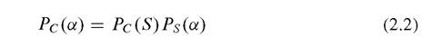
As Luce (1959) proved, this condition is necessary and sufficient to derive the relation:
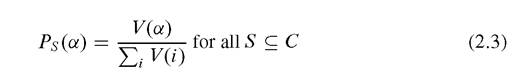
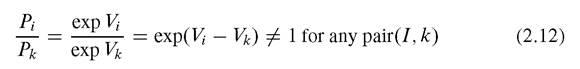
This confirms the existence of a real function with a value V : C → R. It is also verified that function V is unique up to a proportional factor λ ∈ R. That is to say, it holds that:
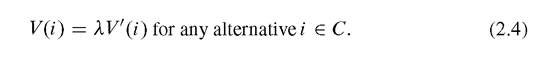
The function V is a Luce-type utility function. Now we substitute eμv≈ for v(a), and eμ-v? for v(β). It immediately follows that:
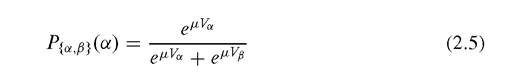
This gives the probability of the decision of a in the subset {a, βg. This expression is useful for estimating an actual mode choice in a group.
We regard a mode as a set of similar types. The mode of a Chinese meal contains many types of dishes with different qualities. A mode may therefore be regarded as an aggregate commodity, by eliminating differences of type due to empirical reasons.[28] Instead of this kind of rounding difference, we could take into account the mode factors (variables) in terms of common measures like time or cost (price).
This idea is immediately applied to an interpersonal framework for choice distribution in society.
In our new environment, we are used to several alternative modes for a particular choice, as well as some alternatives of choice qualities. In short, an individual is allowed to choose a particular mode with his preferred quality.Table 2.1 A mode choice example 1
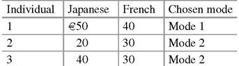
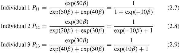
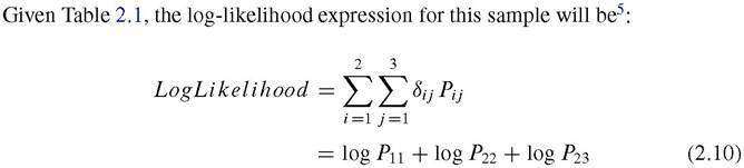
In our cuisine mode example, we can consider a simple numerical example of two alternative modes and three people. The meal could be either of two alternative modes {mode 1, mode 2} = {Japanese, French}. We then employ the univariate case, i.e., cost as a single variable.[29] [30] In other words, we presume the deterministic portion of our utility function as follows: The three people are then faced with a list of different prices (cost variable) in each mode (see Table 2.1). According to Luce’s model, a probability Pi∙j∙ is interpreted as the choice probability for a particular person of choosing a menu type j at mode i. Hence it follows that: Wethen look for the maximum of this function of β, found at β* = 0.0693l47.This is judged as the most plausible in the observed distribution of mode selections in society. Hence we substitute β* into the expressions 2.7-2.9 to get the probabilities (utilities) of mode choice for particular individuals. These arguments have been of much practical interest to policy makers. For example, the choice of travel modes problem is very well known. Given the possible means of transport, {train, bus, plane, car}, a traveler can solve the problem of the desirability of each possible mode to travel to his destination. To make utility maximization feasible, these conditions are required on the deterministic part Va: Reproducibility (consistency): This implies the same choice selection will be made repeatedly under identical circumstances. Acyclicity (a weaker transitivity): This implies a weaker transitivity on preference. Each error term is independent. We also require independence from irrelevant alternatives (IIA). which indicates its independence from the number or attributes of other alternatives in the choice set. In other words, each line must not be mutually proportional among different modes. The limitation of the multinomial logit (MNL) model then results from the assumption of the independence of error terms in the utility of the alternatives. Assume that the choice probabilities (for an individual ora homogeneous group of individuals) are 65 %, 15 %, 10% and 10% for drive alone, shared ride, bus and light rail, respectively. If the light rail service were to be improved in such a way as to increase its choice probability to 19 %, the MNL model would predict that the shares of the other alternatives would decrease proportionately, decreasing the probability for the drive alone, shared ride and bus alternatives by a factor of 0.90 (Koppelman and Bhat 2006, p. 165). 2.1.3