Some Generalizations on Random Terms, Heterogeneities, and Social Interaction

We can decompose the utility on the alternative a into the deterministic part Va and the random term e_α, which then allows us to develop the utility function V to a more general U.^6,7

⁶This part was firstly written in Japanese: Aruka (2004b, pp.

⁷See, for example, Durlauf (1997).

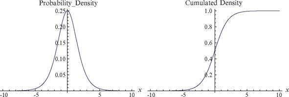
Fig. 2.1 PDF and CDF of a logistic distribution. Note: Here η is set as 1

In the choice set is C = {a, β}, the binary choice. This might, for example, mean an individual i choosing to be either a musician to guarantee the utility V_a or a doctor to guarantee Vβ. However, this choice is likely to be affected by events; for example, attending a gig by a favorite band. Each alternative will be influenced by the random terms e_a,eβ. The binary choice probability of a is then given by:

If we limit the binary choice, we can assume that the next choice set will be:

A particular choice will be realized by a probabilistic distribution of random shocks. We assume a logistic distribution within a particular z of the probability of the random shocks on a binary choice e_i (—1) — ∈i(1) for individual i.

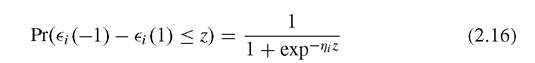
On the choice plane X_i for i, we distinguish the observable characteristics from the unobservable heterogeneity η_i. Here η_i = η(X_i) > 0.

Individual i has his own belief about the choices of the other members of the group I based on information received, F:

Individuals are inclined to either conform to or deviate from the choices of others in the group.^[31] When all the members make the same choice, social utility for any one individual is zero. When they all deviate, according to the Ising model, the social utility for agent i is negative:

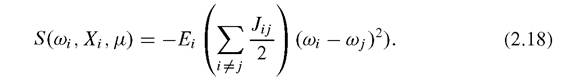
The weight of the interaction Jj (X_i) on the domain of observable characteristics X_i is denoted by Jij, relating the choice for i to that for j. (ω_i — ωj)² will then give the conformity effects. Social utility S is a subjectively expected value based on individual i's belief about the distribution of social interaction [J_j∙ (X_i)].

The decision process of individual i is therefore:

It is easy to derive the solution ω_i by linearization of utility function U. We assume that:

h_i and κ_i are such that:

Since the random shocks are assumed to be subject to the logistic distribution, the probability distribution of the choice of individual i, i.e., ω_i, can be solved:

Thejoint probability distribution of the whole population of the choice of ω is then:

This solution is underpinned by certain limited assumptions including linearization of the utility function and a special form of the error distribution. By introducing

Fig. 2.2 The framing image of random preference.

Source: Aruka (2007, Fig. 2; 2011)

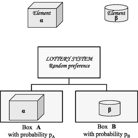
randomness, heterogeneity, and social interaction, however, it may be possible to predict a macroscopic motion to abandon individual subjectivism, moving away from a shortsighted focus on intrinsic preferences. In Fig. 2.2, we show the framing image of random preference. Intermediating by a “lottery system”, we may be taken into either parallel world.

2.1.4