The effect of economic growth on social structures: Empirical evidence
The preceding analysis suggested various channels through which growth is affecting social structures: (a) by shifting individuals from one sector or socio-economic group to another; (b) by modifying income differentials across sectors and socio-economic groups; (c) by modifying income and welfare disparities across individuals.
Of course, these three channels are not independent. In particular, it must be clear that sectoral shifts and inequality changes between socio-economic groups have a direct impact on inequality among individuals.This section briefly reviews the empirical evidence available on these three channels. Both on a cross-country and case study basis, the sectoral shift effect of growth turns out to be the fundamental way through which economic growth affects social structures. Cross-country analysis is less conclusive about the differential effects of growth across socio-economic groups or among individuals. However, this certainly does not mean that growth has no impact on social structures outside the sectoral shift component. Rather, case studies suggest that this effect is more complex and most likely strongly country-specific.
3.1. The sectoral shift effect of growth on social structures
Two rows in Table 1 illustrate the power of growth-related sectoral shift to influence on social structures. Urbanization and all the phenomena that it entails is the first example. The structural explanation behind it is clear. It has to do with the falling share of agriculture - or, better said, of low-productivity traditional agriculture - throughout the growth process. Although only a reduced form model appears in Table 1, coefficients shown there are strongly significant, and it would be relatively easy to devise a structural model focusing more on the mechanisms behind the urbanization process with equally strong statistical significance.
A second sectoral shift effect of growth shown in Table 1 concerns education. Here again, the positive correlation with development levels is very strong. It is true that the coefficient obtained with decadal differences is not statistically significant, but this might have to do with the extremely long lags with which changes in schooling behavior, possibly generated by economic growth, spread to the whole population.[447] It is also true that focusing on literacy rates yields a perspective on education and skills that may seem too narrow. However, it is unlikely that considering the proportion of ‘skilled workers’ in the labor force - assuming that some uniform definition of skills is available across countries - or the proportion of people with secondary education would yield very different qualitative results.[448] In effect, regressing the average number of years of schooling of individuals in the labor force on GDP per capita in Table 1 yields results qualitatively similar to the regression on literacy rate.
One could undoubtedly multiply regressions showing strong structural effects of economic growth through which changes in social structures are likely to occur. For instance, one could focus on the weight of the manufacturing or the service sector instead of focusing on agriculture, or one could focus on the relative weights of low- and high- tech industries or enterprises. Interestingly, this kind of approach to growth - which was prominent in the 1970s, as a continuation of Kuznets research program on ‘modern economic growth’ and under the impulsion of Chenery and associates[449] - is presently weakening. There are various reasons for this neglect, in particular for developed countries as will be seen below. Yet, it would be wrong to conclude from this relative lack of interest that sectoral shift phenomena have disappeared from the research agenda when analyzing the social effects of growth. Indeed, the whole recent literature on the skill bias in the sources of growth and, in particular, technical progress or international trade [see, for instance, the survey by Katz and Autor (1999) and Baldwin and Cain (2000)] may be considered as an updated sectoral shift argument in the analysis of growth and its effects.[450]
Changes in female labor force participation may also be considered as a sectoral shift phenomenon.
But it may also be considered as deriving from a change in behavior itself caused by economic growth. According to the sectoral shift logic, women would be moving from being ‘inactive’ or more exactly specialized in low-productivity domestic production to market employment at a higher level of productivity. According to the behavioral interpretation, the role of women would have been changing in a way concomitant with growth but under forces of a different nature. For instance, some authors see an explanation of the increased female labor force participation in most developed countries after World War II as resulting from the excess demand in the labor market that developed during the war and that had to be filled, a phenomenon that produced a durable change in behavior. Others would insist that the drop of fertility, partly due to the diffusion of contraceptive means in the last three decades or so, was the reason behind women’s increased labor force participation.[451]The preceding phenomena may well provide a partial explanation for the fast increase in female labor force participation in the developed world over the last 60 years or so. However, regressions in Table 1 reveal a rather strong association between participation and economic growth that is not due to cross-country differences, whereas both the fertility and the World War II argument would suggest that those cross-country differences should dominate. Pure cross-country regressions in the first columns of Table 1 yield insignificant results or wrongly signed coefficients when participation is specified as a linear function of GDP per capita. On the contrary, strongly significant results are obtained when within-country time behavior of participation and GDP per capita is taken into account. The simple structural argument that increased female labor force participation may correspond to a shift from low- to higher-productivity occupations is not undermined by the data. Interestingly enough, the same difference between cross-country and within-country estimates appears when participation is regressed on a quadratic form of GDP per capita.
A U-shaped relationship is obtained when not controlling for country fixed effects, whereas a monotonic relationship holds in the opposite case.[452]For the sectoral shift effect of growth on social structures to be of relevance, it is necessary that it takes place between sectors or socio-economic groups with sufficient initial important differences in terms of welfare level. This is certainly the case for the shift across skill (or education) levels, between traditional agriculture and the modern sector of the economy in developing countries or between inactivity and market work for women. Things are less clear in the case of sectoral shifts in developed countries when markets function smoothly and tend to equalize returns of human capital across occupations or sectors. Most likely, this is the reason why this dimension is somewhat neglected in the recent growth literature in developed and emerging countries. The attention there tends to concentrate on differences in the evolution of returns to assets and in their accumulation rather than their sectoral allocation.
The previous remark illustrates possible differences across countries that are hidden by the cross-country work that has been referred to. That differences do exist between developed and developing countries in terms of the social consequences of sectoral shifts of population due to growth is obvious. In Table 1, these differences often are accounted for through the Cox transformation on the dependent variable. But other country differences might exist so that one would ideally like to estimate sectoral shift equations using national time series rather than a cross-section of countries. To some extent, this country specificity is what Chenery and his associates were after when they tried to identify ‘patterns of development’ among developing countries. Unfortunately, due to lack of adequate data, they most often had to rely on calibrated structural models rather than time series structural econometrics.
The situation has changed little since then.3.2. Effect of growth on inequality between socio-economic groups
As mentioned above, the sectoral shift effect of economic growth is important to explain social structures inasmuch as it is accompanied by a persistent differential between socio-economic groups or sectors, in terms of current of permanent income or welfare level. At the same time, it may be envisaged that economic growth contributes to a deepening, or on the contrary, to a weakening of this social differentiation. In effect, those two evolutions are certainly not independent. Sectoral shifts need income differentials to develop and, in turn, they produce changes in these differentials. This subsection focuses on the potential effects of growth on earnings or income differentials across socio-economic groups. Given the dualism with the sectoral shift argument, we adopt the same presentation as in the previous subsection and consider in turn income differentials between sectors - essentially agriculture and the rest of the economy, between skills or educational levels, and between genders.
3.2.1. Sectoral income differentials
The regressions in Table 1 illustrate the fact that sectoral productivity - and presumably income - differentials tend to diminish with economic growth. Thus, growth contributes to harmonize social structures across sectors. The process behind this is clear and has indeed very much to do with the sectoral shift process. As growth proceeds and high- productivity activities arise, people tend to leave low-productivity occupations predominantly located in traditional agriculture. But, this migration process contributes to increasing productivity and income in the sector of origin - and possibly to lower income growth in the sector of destination. The ‘dualism’ of the economy, emphasized by early development economists, tends to diminish with growth. It eventually vanishes when the economy is more mature and market mechanisms ensure the equalization of productivity and earning rates across sectors.
At early stages of development, the preceding process is undoubtedly a powerful source of changes in social structures. At later stages, the emphasis on the agricultural sector is probably ill-placed. A comparison between informal and formal (nonagricul- tural) sectors would be more appropriate. If comparable data were available across countries on this formal/informal distinction, they would probably show a similar phenomenon, that is a narrowing of productivities and incomes across sectors as the informal sector loses weight. At some point, however, the issue becomes essentially that of the functioning of the labor market. The difficulty then is to identify whether earning differentials are due to some segmentation of the labor market or correspond to the self-selection of individuals across jobs with different characteristics and productivity levels.[453] Undoubtedly, these differences raise important social issues regarding the social status differential of workers linked to workers’ social status. But they are of a nature different from the social transformations taking place at earlier stages of development, and it is not clear whether they may be unambiguously associated with growth.
3.2.2. Effect of education on earnings
In a competitive factor market environment, it was argued above that differences in productive asset bundles owned by individuals would be a better indicator of social differentiation than the sector of occupation. Education was thus seen as an important dimension of social differentiation. In this context, the sectoral shift analysis coincides with the change in the distribution of the population, or possibly the labor force, in terms of educational levels. It is now time to examine whether earning differentials across educational groups - often assimilated to skill groups - tend to change in a systematic fashion with economic growth.
There is a huge literature on earning differentials by educational or skill levels and their evolution over time. This is not the place to summarize it.[454] There is considerably less literature on comparing differentials across countries. To our knowledge, the main contributor in this area is Psacharopoulos, who devoted very much effort to the collection of rates of return to education derived from the estimation of Mincerian earning equations based on labor force or household surveys around the world - see in particular Psacharopoulos (1994) and Psacharopoulos and Patrinos (2002). Putting together Psacharopoulos' findings and the lessons from country studies on the evolution of earning differentials leads to some interesting and somewhat paradoxical conclusion. Namely, cross-country comparisons suggest that there is a strong long-run tendency for earning differentials across educational levels to fall, whereas country studies show a very high level of medium-run variability without clear trend.
Table 2 shows mean earning differentials across schooling levels for country groups defined by GDP per capita. These groups cover a total of 98 developed and developing countries for which Mincerian earning equations were available during the period extending from 1970 to 1996, the most recent estimate being used (usually from the late
Table 2
Earning differentials by educational levels (%)
| Primary vs. no schooling | Secondary vs. primary | Tertiary vs. secondary | Average earning differential by year of schooling | |
| Low-income countries | 25.8 | 19.9 | 26 | 10.9 |
| (GDP per capita less than $755) | ||||
| Middle-income countries | 27.4 | 18 | 19.3 | 10.7 |
| (to $9265) | ||||
| High-income countries | NA | 12.2 | 12.4 | 7.4 |
(GDP per capita more than $9265)
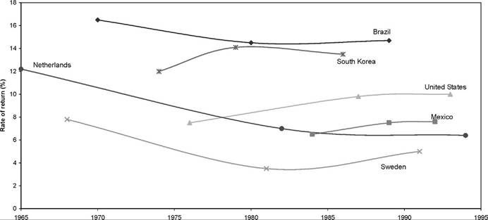
Figure 1. Evolution of rate of return to education (years of schooling). Source: Based on Psacharopoulos and Patrinos (2002).
problems of comparability of samples across countries at different levels of development. In particular, most earning equations are estimated on samples of urban workers. This group of workers represents a high percentage of the labor force in high-income countries, much less in others. Third, the period on which time series are observed may not be long enough to be fully consistent with cross-country differences in development levels.
Finally, there are reasons to expect some time specificity in the evolution of the rate of return to schooling and skill differentials in general. As alluded to before, they are related to Tinbergen’s (1975) idea of the race between technology and education driving the evolution of skill differentials in earnings. For more or less continuous progress achieved on the educational side, it is sufficient to imagine fluctuations or trends in a definite direction in skill-biased technical progress - or possibly in trade policies - to generate time series behavior of the type shown in Figure 1. Alternatively, one may also think of technical progress and its diffusion in the economy following a continuous - not necessarily linear - trend and the educational response intervening with a different time profile to generate various patterns in the evolution of the rate of return to schooling.[455]
For all preceding reasons, it is not contradictory to infer from existing evidence that, indeed, a narrowing of skill differentials and a fall in the rate of return to education is accompanying growth in the long-run, at least in the early stages of development. At the same time, however, this trend may be hidden for long or short periods by accelerations of skill-biased technical progress, major changes in the international trade environment of a country, and velocity of the supply response to changes in skill differentials.
28
3.2.3. Gender earnings differentials
The examination of evidence on gender gaps in individual earnings leads to conclusions opposite to the preceding ones. There, one observes a rather clear downward trend in most countries, although information is scarce for developing countries. By contrast, cross-country comparison points to no systematic differences between countries ranked by development level.
There are relatively few cross-country comparisons of male-female earnings differentials in the literature except for developed countries. Terrell (1992) collected estimates on male-female earning differentials from the ILO Yearbook of Labour Statistics. She found very much cross-country variability, and more importantly as much variability within low- and middle-income countries as within high-income countries. For instance the female-male earnings ratio varied from 0.60 to 0.85 in developed countries, and from 0.50 to 0.90 in developing countries. Of course, the problem is that the samples on which these ratios are evaluated, typically salaried urban workers, differ quite substantially across countries. Thus, the comparison may be of little relevance between a country where 80% of both men and women are in that group and countries where only 20% of men and still a lower proportion of women qualify. This is what explains the paucity of cross-country comparisons encompassing the whole world. Better comparisons can be performed using indirect indicators of earnings. For instance, the regression on male-female difference in literacy rates in Table 1 shows a steady decline with the development level both across countries and across 10-year periods. However, literacy or schooling differences constitute only one among many determinants of earnings differences. Not much is known about gender differences in these other dimensions, nor about their impact on earnings differentials.[456]
In contrast to cross-country, time series of female-male earning ratios available in developed countries show an unambiguous increase over the last few decades. In the US, for instance, this ratio increased from 0.56 to 0.72 between the late 1960s and the late 1990s - see Welch (2000). Comparable increases are observed in European countries.[457] Only a few data points are available for middle-income countries but they reflect a parallel evolution. Between the early 1980s and the mid-1990s, the femalemale ratio among wage earners increased from 0.74 to 0.80 in Taiwan, from 0.62 to 0.72 in Colombia, and from 0.52 to 0.61 in Brazil.[458]
The problem is to know whether such an evolution should be related to economic growth or not. This requires distinguishing between two sources of change in femalemale earnings ratios, one associated with the differential evolution of the characteristics of female and male workers, and the other with changes in the remuneration of these characteristics - i.e. the well-known Oaxaca-Blinder decomposition. In effect, it so happened that the increase in female wage employment concomitant with the previous evolution contributed overall to a lowering of the average skill of employed women in many instances, an effect contributing to a widening rather than a narrowing of the gap. Thus, the observed narrowing must prominently be due to changes in remunerations rather than in the differential characteristics of male and female workers.
The issue then arises of the source of changes in remunerations. Are they related to specific observed characteristics or more diffuse in the whole labor force? In the latter case, it would then be tempting to associate the decline in the female-male ratio to noneconomic phenomena like the evolution of social norms about gender differences, to regulation in the labor markets - minimum wage for instance - or, in some countries, to some kind of affirmative action policies. All these phenomena probably bear some responsibility for the narrowing of the male-female gap, but there also is indirect evidence that it may be due to a change in the remuneration rate of some specific characteristics that distinguish male and female work. This indirect evidence is the positive correlation that has been noted between the female-male earnings ratio and the degree of inequality of male earnings, both in time series - see Blau and Kahn (1997) and Welch (2000) - and in a cross-section of developed countries - see Blau and Kahn (2003). A possible interpretation of that correlation is that changes in male earnings inequality reflect changes in the remuneration rate of earnings determinants, the relative intensity of which happens to differ much between male and female labor. As observed worker characteristics like education or experience do not appear to have played this role, this explanation must rely on unobserved earnings determinants. For instance, Welch (2000) refers to “brains relative to brawn”, with the idea that the relative remuneration of brains in the labor market increases with technical progress, and in effect with economic growth, whereas woman labor is typically more intensive in that factor.
Such an interpretation of the narrowing female-male earnings gap in high-income - and possibly some middle-income countries - is attractive. Yet, it remains to be tested more carefully, a challenging task given that this hypothesis is essentially based on unobserved labor characteristics. At this stage, it is thus difficult to conclude whether it is indeed economic growth that so strongly influences this fundamental dimension of social differentiation. At the same time, it is worth stressing that the preceding issues probably arise only beyond some development level where the labor market is sufficiently unified and competitive. The thinness of the modern labor market and the low weight of women in that market may explain why low income countries are not really comparable to others in terms of gender earnings differentials.
3.3. Effects of growth on inequality among individuals
The preceding subsections looked into how growth affects the structure of the population by sector of activity and by socio-economic groups defined by some observed characteristics, and how it affects income differentials between them. It is now time to consider the possible effect of growth on the overall distribution of income among all individuals in the population. Such a perspective goes beyond the preceding points of view in that it adds to the analysis the possible effect of growth on unobserved individual characteristics through changes in disparities within socio-economic groups. The analysis will proceed in three steps. First, the observed statistical relationship between development levels and income inequality is briefly discussed for a sample of countries and periods where comparable data are available. Second, a more structural approach is discussed where additional variables representing in some way the socio-economic group structure of the population are introduced. Finally, semi-structural studies of the evolution of the distribution in selected countries are discussed. Interestingly enough, the conclusions obtained about the effect of growth on inequality vary rather radically from one approach to another.
3.3.1. Correlation between growth and inequality: rise and fall of the Kuznets curve
As illustrated in the bottom of Table 1, the cross-country evidence on the distributional effects of growth is essentially inconclusive. It is true that a cross-section of countries taken in the 1970s suggests a parabolic relationship that seems in agreement with Kuznets' hypothesis. But cross-sections taken at a later date, and presumably with better data, fail to yield statistically significant results. More importantly, when controlling for country fixed effects so as to isolate the average consequences of within-country growth on distribution, no statistically significant effect can be identified either.
The preceding results fit well the existing literature on the distributional consequences of growth and the Kuznets curve. Back in the 1970s and in the early 1980s, several papers provided pure cross-sectional estimates of the distributional consequences of growth that seemed in agreement with Kuznets' hypothesis, with very much emphasis on the estimation of the turning point at which further growth would cause inequality to go down rather than up - see, in particular, Paukert (1973), Ahluwalia (1974, 1976a and 1976b), Lecaillon et al. (1984). This early literature was very much criticized for its lack of econometric rigor and the quality of the data being used - see, in particular, Anand and Kanbur (1991). When better and more complete data became available, it indeed turned out that the parabolic shape of the relationship between income and inequality was a feature of the 1970s. This feature vanished with the data available in subsequent periods, whereas the first attempts at controlling for country fixed effects confirmed that the findings based on the observations of the 1970s were not robust - see Anand and Kanbur (1993), Fields and Jakubson (1994) and Deininger and Squire (1998), probably the most data-comprehensive analysis available although it relies on secondary data sources.
The interest in the Kuznets hypothesis has not completely vanished today and this hypothesis is frequently revisited in the light of new data and estimation techniques. But the cottage industry that developed around trying to confirm or reject this hypothesis is in decline.[459] At this stage, it seems fair to say that a consensus has emerged according to which available data do not suggest any strong and systematic relationship between inequality and the level of development of an economy. Even those authors who identified a significant relationship agree that it is weak and explains little of the observed differences in inequality.[460]
As in the preceding sections, it may be worth exploring how time series compare to cross-country differences in terms of the correlation between income inequality and development levels. Indeed, considerable attention has been given lately to the evolution of inequality and to the question of whether there was a systematic tendency for modern growth to generate more inequality, as observed in a few countries during the 1980s. This literature is mostly concerned with developed countries because of data availability, even though time series of distribution data in those countries are not always consistent - see Atkinson and Brandolini (2001). The common conclusion of most existing analyses is that inequality has substantially increased in a number of countries between the mid-1980s and the mid-1990s - 12 out of the 17 countries analyzed by Gottschalk and Smeeding (2000). Yet, this evolution must be contrasted with the fact that inequality had been declining in almost all developed countries throughout the 1960s and the 1970s, so that inequality in many countries today is comparable to what it was 30 years ago. It is also worth stressing that inequality failed to increase in a few countries, most likely thanks to very efficient - and possibly increasingly so - redistribution. Time series in developed countries thus seem to confirm the evidence based on cross-country analysis, namely that there is no significant long-run trend, related to the growth process or not, affecting the degree of within-country inequality.
Although data are still more shaky, the same conclusion seems to hold for middle- and low-income countries. Cornia (2001) and Cornia, Addison and Kiiski (2004) find that, out of 34 developing countries for which they have several observations between the 1950s and the mid-1990s, inequality is higher in the terminal period for 15 of them, equal for 14 and lower for 5. Yet, little is said about the intermediate years. When data are available, a U-shape evolution is observed in a number of cases where inequality is found to be increasing when comparing the terminal and the initial years. Overall, clear ascending or descending trends over long periods of time thus are infrequently observed.
Dealing with the effect of growth on social structures, one might prefer to use the concept of poverty, which may have a firmer social connotation than inequality. With this concept, a dimension of social structures is simply the poor-nonpoor difference, that is the proportion of people living in poverty and the distance at which those people find themselves from the poverty line and from the average income of the nonpoor. Of course, if income is taken as the only dimension of welfare, poverty and inequality are rather equivalent concepts when poverty is defined in relative terms, as for instance the proportion of people living with less than 50% of the median income. Poverty, then, becomes a particular inequality measure and much of the preceding argument presumably applies to poverty as well as inequality. Things are different when poverty is defined in absolute terms, as with the widely used international poverty line of $1 a day or any national poverty line representing the minimum budget deemed necessary for survival. Growth then plays a direct role to explain the evolution of poverty. In particular, if the distribution of relative incomes remains constant over time, then changes in poverty essentially reflect uniform income growth in the population. On the contrary, when distribution changes over time, economic growth may play a more complex role depending on its actual effects on distribution.[461] That cross-country analysis fails to find any systematic relationship between distribution and growth suggests indeed that growth has the simpler and more direct impact on poverty that was just mentioned. This is essentially the argument that led Dollar and Kraay (2002) to conclude that ‘growth is good for the poor’. However, it will be seen below that this conclusion may hide considerable disparities across countries.
3.3.2. Towards structural estimates of the effects ofgrowth on distribution?
By focusing on the correlation between inequality and development levels, both in cross-section and time series, the preceding section does not do justice to existing work. Most empirical models that may be found in the literature actually comprise additional variables that may explain the evolution of inequality alongside with, or independently from growth. For instance, the regressions in the pioneer paper by Ahluwalia (1976b) had the income share of various quantiles on the left-hand side and a host of variables on the right-hand side, together with GDP per capita and its square. These variables included the GDP share of agriculture, some educational indicators and some fertility indicators. Thus, the effect of the development level of inequality was supposed to come on top of the effects of sectoral shifts, and associated changes in relative factor rewards. In terms of the analysis in this chapter, the implicit objective of such a specification is somewhat unclear. The distribution between socio-economic groups implicitly defined by variables like the GDP share of agriculture or the degree of urbanization and its impact on overall inequality is taken care of precisely by the presence of these variables in the regression. Under these conditions, the purpose of keeping GDP per capita among the regressors could only have been to identify the effect of economic growth on the distribution of income within those groups, a rather restrictive objective. Retrospectively, the economic framework behind those regressions thus appears as essentially ad hoc, between the reduced form model implicit in the regressions in Table 1 and a true structural model identifying the channels through which growth may indeed affect the distribution. Unfortunately, this imprecision of the economic framework behind the regressions being estimated is rather common in the empirical literature on inequality and development.
Using structural forms in cross-country regressions is possible, but probably requires gathering the appropriate data. In Bourguignon and Morrisson (1990, 1998), for instance, the objective is to explain cross-country differences in distribution explicitly through a model resembling (2) above but with a larger number of assets. Agent’s income is thus taken to be given by
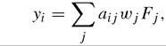
where aij is the share of factor j owned by agent ł, the total endowment of factor j is given by Fj, and Wj is its remuneration rate. Endogenizingthe latter within the framework of a small open economy, it is then possible to write the overall distribution of income {y} as

where the arguments of the function H(∙) are the distribution of resources in the population {a..}, the vector of total endowments F., the vector of international prices faced by the economy p, and the tax rates and tariffs that it imposes t. Then, one may try to proxy for these various arguments by aggregate data available on a comparable basis across countries and use the resulting empirical model to analyze the effects of economic growth on the distribution.
The two papers referenced above stop short of the latter objective, mostly because of the difficulty of identifying all the variables necessary for the analysis and the necessity of using very imperfect proxies, which prevent proceeding with a truly structural analysis. For instance, physical capital per worker is approximated by GDP per capita. This is not unjustified for a given value of other aggregate endowments of productive factors, but this makes it impossible to distinguish the distributional effects of capital accumulation and of total factor productivity. Even so, however, the analysis shed light on the effects of the ownership distribution variables - land, human capital - on the distribution of income at one point of time, as well as on the impact of relative aggregate endowments (land, physical and human capital and raw labor) and policy variables like trade protection. In line with the argument in the previous sections, it also showed
the importance of labor market competitive imperfection, and in particular the ‘dualism’ of the economy as represented by the relative productivities of the agricultural and nonagricultural sectors.
Going beyond these partial results and analyzing the potential effects of growth in the distribution of income within the framework of (8) is still on the agenda. Better data are necessary. As rough as existing empirical applications may be, however, this analysis suggests that the distributional effects of growth are complex and most likely to be strongly differentiated across countries. With the preceding specification and in view of the results obtained, it appears clearly that growth affects the distribution through various channels - changes in relative factor endowments, changes in the distribution of these factors, changes in policies, changes in the functioning of factor markets - and in a way that may depend on the initial value of these various macro-economic characteristics.
3.3.3. Case study analysis
Should one then conclude with Dollar and Kraay (2002) that growth is distributionally neutral and therefore that “growth is good for the poor”, whatever the engine behind it? The preceding argument suggests that it would be going too far. What the important literature on the effect of growth on inequality shows is essentially that there is apparently no significant relationship that would be valid across countries and time periods. It certainly does not say that this is true for specific countries during a particular period. Sizable changes have been observed in several countries in the recent past, the causes of which are not always readily apparent but which are not necessarily independent from economic growth and some of its features.[462] In effect, most case studies on the evolution of inequality over time single out characteristics of the growth process or of policies behind it that are responsible for specific distributional changes. The debate that took place recently on whether recent increases in earnings inequality in various developed countries were due to technical progress and the consequent shift of developed economies towards high-tech is a good example of such an approach.
An important stream of case studies on the distributional consequences of growth is found in the historical literature. Following the example of Kuznets himself, numerous economic historians tried to identify the trend in some inequality measure over long periods of time. Findings often conform with the Kuznets curve hypothesis. Yet, a common problem is that very much of that literature relies on very rough measures of inequality often based on a few macro-economic characteristics and ignores important sources of micro-economic heterogeneity. Because of this, it tends to over-emphasize the role of phenomena like urbanization or the shift away from self-employment - that is, sectoral shift phenomena. A survey of findings is offered by Lindert (2000) and Morrisson (2000).
Identifying empirically the forces through which economic growth may shape the distribution of income in actual growth experiences is a difficult task because it requires correcting the observed evolution of the distribution for sources of change unrelated or very loosely related to growth. An exercise of this type was undertaken in a series of case studies that explore the microeconomics of income distribution dynamics (MIDD) in a small number of middle-income countries.[463] The following example illustrates the difficulty of empirically isolating the distributional effects of growth and shows at the same time the major potential role that growth plays in distributional issues.
The methodology used in the MIDD study consists in decomposing the observed change in the distribution of earnings or per capita income into three types of effects, which parallel the general argument in this chapter. The first type corresponds to changes in the structure of earnings for given socio-demographic characteristics of individuals, and possibly by labor market segment if the labor market is imperfectly competitive. The second set of effects corresponds to a change in the labor supply of individuals or household members, and possibly their allocation across labor market segments. The final set of effects includes those occurring due to a change in the distribution of socio-demographic characteristics of individuals and households. In terms of the analysis in this chapter, the second and third type of effects would, in some sense, correspond to the shift of people across socio-demographic groups, whereas the first one would correspond to changes in income differentials across these groups, a residual term actually included in the third effect, accounting for changes in the distribution within groups. Each effect is estimated by simply substituting in the initial year the characteristics of the final year in one of the various dimensions just indicated, or vice versa. Thus, the effect of the structure of earnings is obtained by simulating what would be the distribution of income in year 1 if the structure of earnings by socio-demographic characteristics (gender, education, region, etc.) had been the one observed in year 2. The ‘fertility effect’ is obtained by importing in the initial year the same relationship between family size and parents’ characteristics (education, age, race, region, etc.) as the one observed in the terminal year, etc.[464]
This methodology has been applied, among other countries, to Brazil during the period 1976-1996.[465] What is remarkable during that period in Brazil is that neither the mean income - or GDP per capita - of the Brazilian population nor inequality changed much, even though most usual aggregate inequality measures show a moderate decline. From this direct observation, one might then conclude that very slow growth was associated in Brazil with virtually no change in the distribution of earnings or income. This would be erroneous, however. What happened is that other phenomena compensated for the distributional effects of slow growth. The decomposition methodology presented above led to 3 conclusions:
(a) Over the period under analysis, family size went down significantly and more so among people with low education and income. Because of this factor, inequality in Brazil should have substantially declined.
(b) The structure of earnings changed moderately against least-skilled and selfemployed workers.
(c) It also turned out that the occupational structure of the population was modified. Employment in general, and employment in the formal sector in particular, had gone down, hitting more severely the segments of the population with the lowest education levels and at ages where access to the labor market is the least easy - young and old people. Overall, however, these various changes tended to compensate each other.
Although the methodology described above does not include any formal representation of the labor market and the way it may be affected by growth, it is difficult not to relate points (b) and (c) to the sluggish growth performance of Brazil during the two decades under analysis. Within a dual economy framework, which seems to fit well the Brazilian economy, the general story would thus be as follows. Slow growth was responsible for a weak labor market, which may have caused an increasing skill differential in the earnings of wage workers and self-employed, as well as job losses or worker discouragement among the least skilled. Both phenomena, but mostly the latter, actually contributed to an increase in inequality. The reason why this inequality increase did not actually show up is that it was compensated by falling family sizes which were more pronounced at the bottom of the distribution - and to a lesser extent progress in the education level of the poorest. Slow growth in Brazil might thus have been responsible for increased inequality after all.
This example shows that identifying the actual effects of economic growth on the social structure of a population may require more than simply observing the changes in that structure and the rate of growth during a given time period. Some of the observed change in social structures may indeed be directly imputed to what is happening on the economic growth front, but may also be due to other concomitant phenomena which are independent of growth or very indirectly related to it. With this example in mind, one may then understand perfectly that the phenomena put forward by economic theory to explain how economic growth is likely to affect social structures may be difficult to observe in actual growth episodes. This is because parallel phenomena, not directly related to growth - but not necessarily independent from it either - affect the distribution and introduce some noise in the observation, both in cross-sectional and time series analyses.
The important point here is that the channels identified by theory may well prove empirically relevant when the necessary correction of available data for other nonneutral distributional phenomena has been made. Of course, the difficulty is to know whether these phenomena are themselves growth dependent or not. In the preceding case, did the change in fertility take place in an autonomous way, or was it the result of economic growth per se, or possibly the result of an educational improvement which itself could have been autonomous or the result of growth? It is this kind of structural model that must be confronted with the data, rather than the very reduced-form models behind cross-sectional work or simple comparisons of changes in inequality and income per capita measures. This is a much more difficult exercise, which has barely begun.[466]
4.