A unified theory of the evolution of international incomes
In this section we unify the Parente and Prescott (2000) theory of relative efficiencies and the Hansen and Prescott (2002) theory of development. The unified theory is then used to organize and interpret the evolution of international income levels.
We unify the Parente and Prescott theory and the Hansen and Prescott theory as follows. We assume that technological level increases in both sectors result from growth in world knowledge. Consequently, the technology component of TFP in each production function is the same across countries at any point in time. The paths for the technology components of TFP are determined as in Section 2.3 by requiring that the leader country with an efficiency parameter in the modern sector set to one start its transition to modern economic growth in 1700. We then introduce differences in this efficiency parameter across countries. Given a country’s relative efficiency parameter and the common path of the technology components of the TFPs, we compute the equilibrium path of the economy.As mentioned in Section 3, we doubt than any country has or had an efficiency parameter equal to one. The assumption that efficiency in the leader is one in the unified theory is not important to any of the results because it is just a normalization. Again, only relative efficiencies matter and can be determined. This is the case for countries at a given time and across time in a given country.
We do not introduce cross-country differences in the efficiency parameter associated with traditional production. As mentioned in the Introduction, incomes did differ slightly prior to 1700, with the richest countries being no more than two or three times richer than the poorest. One possible explanation for these pre-1700 differences in income levels is that countries differed in policies that increased the inputs required for producing goods with the traditional production function.
Because this technology corresponds to traditional farming and even manufactures produced within a home setting, we think the effect of policy differences for relative efficiencies associated with traditional production is small. For this reason, we favor the alternative explanation that some countries were better able to defend themselves from outside expropriations because of geography and thus were able to maintain a higher constant living standard during the pre-1700 era. Two countries that enjoyed such an advantage were England and Japan.We interpret delays in the start of the transition to modern economic growth to late starters having a lower relative efficiency in the modern sector, at least up until the date their transitions began. We attribute the persistent percentage difference between such a country and the industrial leader to the continuation of its low relative efficiency. Finally, we attribute catch-up, including growth miracles, to large increases in relative efficiency in countries.
We begin by computing the relative efficiency of a late starter required to delay the start of its transition by a given length of time. The size of the required efficiency difference between the leader and the laggard that gives rise to any given delay is a function of the capital share parameter in the modern production function. Our main finding is that differences in relative efficiency required to generate delays in starting dates of the lengths observed in the historical data are reasonable for all capital shares above 0.40.
We then compute the entire equilibrium path of these late starters assuming that their efficiency levels relative to the leader never change. Large differences in incomes exist even after the late starters are in the modern economic growth phase. In fact, the gap between the leader and late starters increases for some time after the laggards have started the transition to modern economic growth. This is the case even though the transition period of late starters is shorter than that of early starters.
The main finding of these experiments is that the gap in incomes between early and late starters never narrows unless the laggard adopts polices that increase its productive efficiency.The final set of experiments allows for a one-time increase in a country’s relative efficiency parameter. We assume that the change is unexpected from the standpoint of the late starter and viewed as permanent in nature. We then compute the equilibrium path and determine the country’s output relative to that of the leader subsequent to the change. We find that the late starter’s path of output relative to the leader subsequent to the change in its efficiency parameter is consistent with the experience of growth miracle countries such as Japan, but only if the capital share is between one-half and two-thirds.
We conclude from this analysis that capital’s share must be large for the unified theory to be a successful theory of the evolution of international income levels. A large capital share implies an important role for intangible capital in the production of goods and services and large investment in intangible capital as a fraction of GDP. Investment in intangible capital goes unmeasured in the national income and product accounts. Thus, it is not possible to determine whether a large capital share is plausible by examining national account data. One must examine other evidence, in particular, micro evidence to determine the plausibility of a large capital share. Thus, we end this section by examining the micro evidence on the size of unmeasured investment in the economy. We conclude from this evidence that the size of unmeasured investment in the economy is as large as the size predicted by the unified theory.
4.1. Delays in starting dates
We first examine whether the unified theory predicts large delays in the start of the transition to modern economic growth that some countries have experienced. In particular, we determine the size of the difference in efficiency required to delay the start of the transition to modern economic growth by a certain number of years.
For the purpose at hand, it is important to provide a more thorough picture of the different starting dates for the transition corresponding to the experiences of individual countries. An issue is how to date the start of modern economic growth. Our definition of the start of modern economic growth is the earliest point in a country’s history with the property that the trend growth rate is 1 percent or more for all subsequent time.[264] Fig-
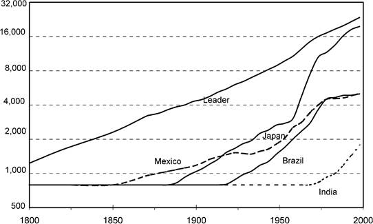
Figure 7. DifFerent countries start at different dates, income per capita in 1990 $US. Source: Maddison (1995).
ure 7 shows the path of output in a number of countries relative to the industrial leader going back to 1800. As can be seen, starting dates vary substantially across countries. Mexico started its transition to modern economic growth sometime between 1800 and 1850; Japan started sometime between 1850 and 1900. Brazil started in the early twentieth century, and India started its transition sometime between 1950 and 1980. Each country's income gap with the leader increased prior to starting its transition to modern economic growth.
The key expression for determining the delay in the starting date associated with differences in relative efficiencies is Equation (3.12), which rewritten in relative efficiencies is

A country will not use the modern production Iiinction as long as the relation given by Equation (4.1) is satisfied. Once a country's efficiency, EsAst, exceeds the critical level given by the right-hand side of Equation (4.1), which it must, the country begins its transition to modern economic growth. Assuming as we do that relative efficiencies associated with the traditional production function do not differ across countries, the rental prices of land and labor will not differ much across countries over the periods when each country specializes in the traditional production function.[265] Consequently, this critical level of efficiency will not differ much across countries.
It follows that the difference in starting dates between two countries i and j, with different relative efficiencies, is approximately given by the periods ti and tj for which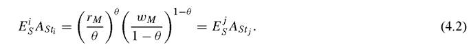
It is not obvious looking at Equation (4.2), but the required relative efficiency Els∕ES that gives rise to a particular delay in the start of the transition depends on the size of the capital share in the modern production function. The reason for this is that the required factor difference in relative efficiencies equals the factor difference in the stock of pure knowledge, As, between starting dates. It follows that the required relative efficiency difference is smaller for larger increases in the stock of pure knowledge between starting dates. The size of the increase in the stock of pure knowledge depends importantly on its asymptotic growth rate γs. The value of this parameter is calibrated so that the growth rate of per capita output associated with the constant growth path of the modern-growth- only model, given by (1 + χs)1^1-^, equals 2 percent per year. Thus, the calibrated value of γs, and hence the implied size of the factor increase in pure knowledge between starting dates tj and ti, depends on capital’s share in the modern growth production function.
We now compute the efficiency of the early starter relative to a late starter required to generate a given delay in the transition to modern economic growth. We do this for a range of values for the capital share parameter, since the value of capital’s share is not well restricted. For each capital share value, we recalibrate the asymptotic growth rate of pure knowledge γs and the value of As0 so that the country with Es = 1 always starts its transition in 1700. These are the only parameters whose values are changed in the experiments.
We assume that late starters are endowed with an initial capital stock equal to the steady-state level associated with the classical model of Section 2.1. For the purpose of determining the date at which an economy starts to use the modern growth function, it is not necessary that we fully specify the population growth function of the late starters. In particular, it is not necessary to specify the population growth function for consumption levels sufficiently greater than the constant consumption level, cm, associated with the pre-1700 period. For consumption levels below this, we use a population growth function with a sufficiently large and positive slope at cM and for which g(cM) = (1 + óě)1/(1~ô~^). Theseassumptionsensurethatthelivingstandardinalate starter is roughly constant prior to the period it begins its transition.
Table 2 reports the efficiency of the early starter relative to the late starter required to generate a 100-year, a 200-year, and a 250-year delay in the transition to modern economic growth. These delays roughly represent the difference in the start of the transition to modern economic growth between England and Mexico, England and Japan, and England and India. As Table 2 shows, the factor difference in efficiency needed for a given delay decreases as the capital share in the modern production function increases. The size of the required difference needed to delay the start of development for
Table 2
Required factor difference in relative efficiencies for delays
| θ | 1800 start | 1900 start | 1950 start |
| 0.40 | 1.60 | 3.2 | 5.7 |
| 0.50 | 1.25 | 2.5 | 4.0 |
| 0.60 | 1.20 | 2.2 | 3.3 |
| 0.70 | 1.18 | 1.9 | 2.5 |
250 years is plausible for all values of θ in Table 2, with θ = 0.40 probably at the lower bound of plausible values.
4.2. No catch-up after the transition in many countries
A number of countries, many of which are located in Latin America, began modern economic growth toward the end of the nineteenth century. By and large, these countries have failed to eliminate the gap with the leader over the twentieth century. We now examine whether the model can account for this feature of the data. In particular, we seek to determine if the model predicts a narrowing of the gap between a country’s income level and the level of the leader once that country begins the transition to modern economic growth.
We address this question by examining whether the model absent any subsequent changes in relative efficiencies predicts a narrowing or widening of the gap between income levels between early and late starters. In particular, we compute the equilibrium paths of per capita output over the 1700 to 2050 period for the model economies associated with the required differences in relative efficiencies listed in Table 2. We also report their asymptotic income levels relative to the leader.
Before undertaking these experiments, it is necessary to address two issues. First, it is necessary to specify the population growth rate function for the late starters in these experiments because increases in population affect the size of the increases in per capita output over the transition. For this specification, we simply use the post-1800 population growth rates of Mexico for the model economy that starts its transition in 1800, the post-1900 population growth rates of Japan for the model economy that starts its transition in 1900, and the post-1950 population growth rates of India for the model economy that starts its transition in 1950. These population growth data are taken from Lucas (2002, Table 5.1). Second, for capital share values that reflect a broad concept of capital, it is necessary to adjust output by the amount of investment in intangible capital. This adjustment must be made in order to compare the predictions of the model with the national income and product accounts, because the latter fail to measure investments in intangible capital. Thus, GDP in the national accounts corresponds to Y — Xj in the model economy.
A country’s unmeasured investment as a fraction of its measured output can be determined given the decomposition of the capital share between its physical capital and intangible capital components. For a given total capital share, the physical capital component can be calibrated to the ratio of investment in physical capital to measured GDP in the leader countries of roughly 20 percent. In particular, the individual share parameter values can be calibrated to the steady state of the modern growth-only economy using this observation from the leader countries.
With values of the individual share parameters in the modern growth production function in hand, it is possible to compute the amount of unmeasured investment in any period along an economy’s equilibrium path. Table 3 reports the size of the intangible capital share parameter and the asymptotic ratio of intangible capital investment to GDP for each of the total capital share values considered in Table 2. As the total capital share increases, both the intangible capital share and the intangible capital investment share of GDP increase. The sizes of the unmeasured investment shares range from 0.0 for θ = 0.40 to 0.62 for θ = 0.70.
Figure 8 plots the path of per capita GDP for late starters relative to the leader over the 1700-2050 period. The paths correspond to the case where θ = 0.40. The paths are essentially the same for the other capital share values. For reasons of space, they are omitted in this chapter. Asymptotically, the model is just the steady state of the modern growth model of Section 2.2, and so income differences are just (Ets∕Ejsy(1~θ). For the 1800 starter, the asymptotic relative income level is 50 percent of the leader, for the 1900 starter, it is 16 percent, and for the 1950 starter it is 6 percent.
Most of the difference in relative incomes in 2000 is the consequence of the poor country starting the development process later. However, even after starting to develop, a late starter’s disparity with the leader increases, although at a much slower rate than before. There are two reasons for this. First, the disparity continues to increase because the traditional production function is still widely used at the start of the transition and the growth rate of TFP associated with the traditional production function is lower than the growth rate of TFP associated with the modern production function. Second, the population growth in these countries tends to be higher compared to the leader over the comparable period. The disparity with the leader stops increasing only after the modern production function starts being used on a large scale. For the 1800 starter, the disparity stops increasing around 1900. For the 1900 starter, the disparity stops increasing
Table 3
Implied intangible capital share and investments
| θ | θι | Xi/(Y - Xi) |
| 0.40 | 0.00 | 0.00 |
| 0.50 | 0.28 | 0.26 |
| 0.60 | 0.41 | 0.41 |
| 0.70 | 0.53 | 0.62 |
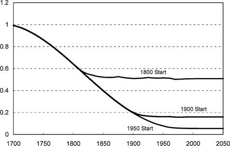
Figure 8. Predicted income per capita relative to the leader.
around 2000. And for the 1950 starter, the disparity stops increasing around 2050.[266] The increase in disparity over the 1950-2000 period for the 1950 starter is consistent with the fact that many sub-Saharan countries have fallen further behind the leader in the 1950-2000 period despite experiencing absolute increases in living standards over this period.
Laggards do experience larger increases in their income over their transition periods compared to earlier starters. For example, the country that starts its transition in 1700 realizes a factor increase of 1.2 in its per capita income by 1750. In comparison, the country that starts its transition in 1900 realizes a factor increase of 2 in its per capita income over the next 50 years.[267] The reason for this difference is that the growth rate of knowledge associated with the modern production function is initially low, but rises over time. Thus, TFP growth in the modern production Iiinction over a late starter's transition period is higher than an earlier starter's transition period. This gives late starters an inherent advantage.
The data needed to verify whether this pattern exists are not readily available because per capita income estimates going back to the eighteenth century exist for only a limited number of countries. Thus, it is not possible to say whether transition periods have become shorter over time. There is, however, strong evidence that late starters have been able to double their incomes in far shorter time periods than earlier starters.
Figure 9 documents this general pattern. It plots the number of years a country took to go from 10 percent to 20 percent of the 1985 U.S. per capita income level versus the first year that country achieved the 10 percent level. The 1985 U.S. level was 2,000
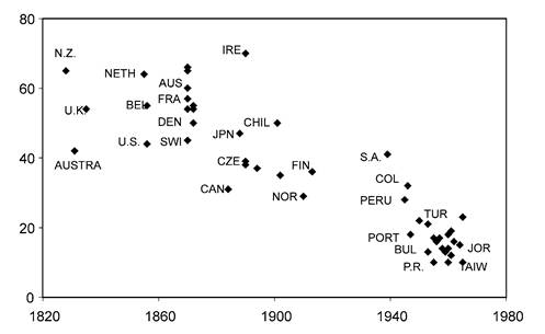
Figure 9. Years for income per capita to grow from 2,000 to 4,000 (1990 $US). Source: Maddison (1995) and Summers and Heston (1991).
in 1990 dollars. The set of countries considered had at least 1 million people in 1970 and had achieved and sustained per capita income of at least 10 percent of the 1985 U.S. level by 1965. There are 56 countries that fit these criteria and for which data are available. Of these 56 countries, all but four managed to double their per capita income by 1992. The four exceptions all had protracted armed insurgencies that disrupted their development.
The difference in the length of the doubling period between the sets of late and early starters is dramatic. For early starters, which are those achieving 10 percent of the 1985 U.S. level before 1950, the median length of the doubling period is 45 years. For late starters, defined as those achieving 10 percent of the 1985 U.S. level after 1950, the median length of the doubling period is 15 years. The choice of starting level is not important. A similar pattern emerges when the starting level is fixed at 5 percent and at 20 percent of the 1985 U.S. level.
Although the model absent changes in relative efficiency infers an advantage to late starters, quantitatively it is inconsistent with the number of years in which many late starters have been able to double their income. Many late starters that doubled their income in less than a 35-year period after 1950 did in fact narrow the gap with the leader over that period. The unified theory absent changes in relative efficiencies does not predict any catch-up for late starters. For the theory to account for this catch-up, it must consider changes in relative efficiency in a given country over time.
4.3. Catch-up and growth miracles
We now examine whether the theory can account for the record of catch-up. A key feature of the evolution of international income levels is that many countries have been able to narrow the gap with the leader, with some realizing large increases in output relative to the leader in a relatively short period of time. A number of countries, primarily located in Western Europe, caught up to the leader in the post-World War II period. A number of other countries primarily located in Southeast Asia eliminated a large fraction of their gap with the leader in this period. Some of these countries had miraculous growth experiences doubling their living standards in less than a decade in the post-1950 period. These growth miracles are a relatively recent phenomenon and are limited to countries that were relatively poor prior to undergoing their miracle. No country at the top of the income distribution has increased its per capita income by a factor of 4 in 25 years, and the leader has always taken at least 80 years to quadruple its income.
To account for the catch-up, including growth miracles, the theory requires an increase in the efficiency of a country relative to the leader.[268] In light of the Parente and Prescott (2000) theory, these changes in relative efficiency are easy to understand. Namely, they reflect policy changes. Following an improvement in policy that leads to a significant and persistent increase in efficiency, the theory predicts that the income of a late starter will go from its currently low level relative to the leader to a much higher level. As it does, its growth rate will exceed the rate of modern growth experienced by the leader, and the gap between its income and the leader’s income will be narrowed.
We now consider an increase in a late starter’s relative efficiency. In particular, we examine whether the unified theory can account for the growth miracle of Japan. Figure 10 depicts the path of per capita output for the Japanese and U.S. economies over the 19001995 period. There is really nothing special about Japan relative to other economies that similarly experienced growth miracles. It would have been just as easy to study the cases of other growth miracle countries such as China, South Korea, and Taiwan in this experiment. The precise time period of the Japanese growth miracle we consider in the analysis is the 1957-1969 period. We choose this period because by 1957 Japan had fully recovered from the wartime disruptions. Moreover, this period is one of the most dramatic in terms of Japan’s catch-up. In this 12-year period, per capita GDP doubled from 25 percent of the leader to 50 percent of the leader. [See Summers and Heston (1991).] This catching-up was not the result of the leader’s growth rate slowing down. Indeed, U.S. per capita GDP grew by 40 percent in this period. The Japanese economy in this period is a dramatic example of catching up.
The experiment assumes an unexpected increase in 1957 in the relative efficiency of the model economy, which started its transition in 1900, to the level of the leader. This assumption is made because the data suggest that Japan in the 1957-1969 period was converging to the U.S. balanced growth path. In calculating the equilibrium path of the model economy following this increase, we take the initial population to be the population corresponding to the equilibrium path of the model economy that starts the transition in 1900. The initial capital stock is assumed to be such that per capita GDP
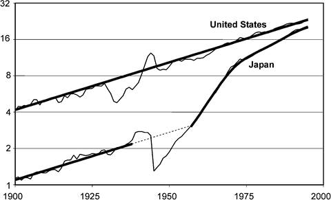
Figure 10. Income per capita 1900-1995 (1990 $US). Source: Maddison (1995) and Summers and Heston (1991).
relative to the leader equals 25 percent.[269] The population growth rate function for the model economy is the same as before and is based on Japanese population dynamics.
The important finding is that the total capital share must be large for an economy to take 12 years to move from 25 percent to 50 percent of the leader. Figure 11 plots the path of per capita GDP predicted by the model economy over this period for various values of θ. For a value of θ equal to 0.40, the predicted path shows too large an increase over the period. At the other end of the range, namely, θ = 0.70, the predicted path shows too small an increase over this time period. This leads us to conclude that capital share values in the range from 0.55 to 0.65 are consistent with growth miracles.[270]
It is possible to introduce this increase in efficiency in the poor country at a much earlier date, say in 1800. The theory does not, however, predict that the poor country will experience a growth miracle. The theory, therefore, is consistent with the fact that growth miracles are a relatively recent phenomenon. Growth miracles are a relatively recent phenomenon because, as Figure 8 shows, differences in relative incomes between the low-efficiency and high-efficiency countries widen over time before leveling off. This widening is due to growth in the stock of pure knowledge associated with the modern production function, which the high-efficiency country uses from a very early date. Thus, as one goes back in time, the gap that a low-efficiency country could close by becoming a high-efficiency country becomes smaller and smaller. Obviously, if the gap is less than 50 percent, the low-efficiency country could never double its income in less than a decade. For the same reason, the unified theory is consistent with the fact
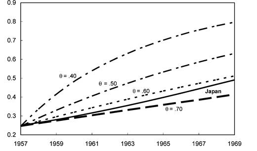
Figure 11. Growth miracles: income per capita as fraction of the leader. Source: Summers and Heston (1991).
that late starters have been able to double their incomes in far shorter times compared to early starters.
The theory is also consistent with the fact that growth miracles are limited to countries that were initially poor at the time their miracles began. Growth miracles are limited to this set of countries because a growth miracle in the theory requires a large increase in a country's relative efficiency. A large increase in efficiency can only occur in a poor country with a currently low efficiency parameter. This rules out a rich country, which by definition uses its resources efficiently, from having a growth miracle.
4.4. Unmeasuredinvestment
For capital share values that are consistent with the evolution of international income levels, the implied size of unmeasured investment is between 35 and 55 percent of GDP. An important question is whether these intangible capital investment share numbers are plausible. This is not an easy question to answer. The difficulty in coming up with measures of the size of intangible capital investment is that the national income and product accounts (NIPA) treat investments in intangible capital as ordinary business expenses. Such investments, therefore, are not measured.
To better understand this, consider the case where a firm hires computer instructors for $100 to train its workers to use the latest software. This expenditure of $100 by the firm clearly represents an investment in the stock of intangible capital. It is not included in GDP in the national accounts. In terms of the national accounts, the $100 is the payment to the instructors, and so enters the income side of the national accounts under compensation to employees. However, since the expenditure is treated as an ordinary business expense, the firm's accounting profits are lowered by $100, and corporate profits in the national accounts are lowered by $100. These entries exactly offset each other so the transaction has no effect on either the income side or the output side of the national accounts. The investment in intangible capital, thus, goes unmeasured.
Parente and Prescott (2000) attempt to estimate the size of intangible capital investment in the U.S. economy by examining micro evidence of the size of the investments that firms and people make in intangible capital. In constructing their estimates, Parente and Prescott (2000) use the principle implied by theory that investment is any allocation of resources that is designed to increase future production possibilities. Using this principle, they identify such activities as starting up a new business, learning-on-the- job, training, education, research and development, and some forms of advertising as investments in intangible capital.[271] They conclude that the size of this investment may be as large as 50 percent of GDP. Such estimates are consistent with capital share values between one-half and two-thirds.
5.