A theory of relative efficiencies

The Hansen and Prescott (2002) theory of economic development reviewed in Section 2 is not a theory of the evolution of international income levels. It does not address the issue of why modern economic growth started at different dates in different countries.

One might be led to introduce differences in TFP associated with the modern pro­duction function to the model, because the Hansen and Prescott theory of development predicts that per capita income in a country starts to increase once TFP in the mod­ern sector reaches a critical level. Moreover, there is ample evidence that countries (at least those experiencing modern economic growth) differ along this dimension.^[260] Al­though it would be easy to introduce such differences into the Hansen and Prescott theory, it would not be useful, as long as country-specific TFP differences are treated exogenously.

Parente and Prescott (2000) develop a theory of TFP that attributes differences in TFP to country-specific policies that both directly and indirectly constrain the choice of production units. Their theory of TFP is more appropriately called a theory of rel­ative efficiencies. This is because Parente and Prescott (2000) decompose a country’s TFP into the product of two components. The first component is a pure knowledge or technology component, denoted by A. The second is an efficiency component, denoted by E. In the context of the Hansen and Prescott model, the modern growth production function is

The technology component of TFP, A_St, is common across countries. It is the same across countries because the stock of productive knowledge that is available for a coun­try to use does not differ across countries.^[261] The efficiency component differs across countries as the result of differences in economic policies and institutions. Here we consider the case in which a country’s economic policies and institutions do not change over time, so E_s is not subscripted by t. The efficiency component is a number in the (0, 1] interval. An efficiency level less than one implies that a country operates inside the production possibilities frontier, whereas an efficiency level equal to one implies that a country operates on the production possibilities frontier. Differences in efficiency, therefore, imply differences in TFP.

Relative efficiencies at a point in time, and not absolute efficiencies, can be deter­mined using the production function and the data on quantities of the inputs and the output. Thus, it is not possible to determine if any country has an efficiency level equal to one, although we tend to doubt that this is the case.

We now present the Parente and Prescott (2000) theory of relative efficiencies. To keep the analysis manageable, we present the theory of relative efficiencies in the con­text of an economy in which only the modern production function is available. The theory constitutes a theory of the aggregate production function when there are con­straints at the production unit level.

In light of this, we first review the theory underlying the aggregate production func­tion. We then show how policy constraints give rise to an aggregate production function with a different efficiency level. We follow this by providing estimates of cross-country relative efficiencies associated with the modern production function using the mapping from policy to aggregate efficiency derived in this section with estimates of the costs im­posed by a country-specific policy. Finally, we conclude this section with a discussion of why constraints on the behavior of the production units exist.

3.1. The aggregate production function

Before developing the mapping from policy to aggregate efficiency, we briefly review the theory of the aggregate production function associated with modern growth. The the­ory underlying the aggregate production function is as follows. In each period, there is a set of plant technologies B. A plant technology b ∈ B is a triplet that gives the plant’s output y_b and its capital and labor inputs, k_b and n_b. A plan {λ_b} specifies the measure of every type of plant operated. The aggregate production function, that is, the maximum Y that can be produced given aggregate inputs K and N is

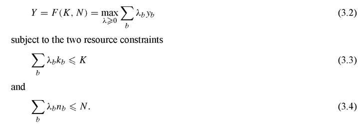
Assuming that this program has a solution, which it will under reasonable economic conditions, the aggregate production function will be weakly increasing, weakly con­cave, homogeneous of degree one, and continuous.

Empirically, the Cobb-Douglas aggregate production function is the one consistent with the post-1900 modern economic growth era. The question then is: What set of technologies B gives rise to the Cobb-Douglas aggregate production function? One such set is the set of plant technologies defined by

The function d(n) is an increasing and continuous function of the labor input. Assuming that n* = argmax d(n)n^θ-1 exists, the aggregate production function is

where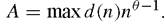A sketch of the proof is as follows. If any quantity of capital

and labor is allocated to a single type plant in such a way that output is maximized, then the number of employees at each plant is n*. Thus, all operated plants, for an optimum, must have n* workers. Given θ < 1, the capital stock must be allocated in equal quantity over every operated plant. Thus, the number of plants operated is N∕n*, capital per operated plant is K∕(N∕n*), the number of workers per operated plant is n*, and maximal output is given by Equation (3.6). With the assumption that the function d increases over time, the expression A will increase over time.

3.2. Consequences of constraints for aggregate efficiency

Next, consider the plant production technology with constraints imposed on it. We con­sider two types of policy. The first type constrains how a particular plant technology can be operated. The second type constrains the choice of which plant technologies can be operated. Certainly, these are not the only types of constraints that will affect a country’s TFP. A number of other types of policy have a similar effect.¹⁷

The first type of policy constrains how a given technology is operated.

the nature of the constraints were to double the capital and labor requirements, then the efficiency measure would be one-half. If the nature of the constraints is to quadruple both the capital and labor requirements, then the efficiency measure would be one- fourth.

The second type of policy constrains the choice of which technology can be operated. This type of constraint maps into the efficiency parameter of an aggregate production function with a composite capital stock made up of both physical and intangible com­ponents. Any policy that serves to increase the amount of resources the production unit must spend in order to adopt a better technology is a constraint of this nature. Such policies and practices take the form of regulation, bribes, and even severance packages to factor suppliers whose services are eliminated or reduced when a switch to a more productive technology is made. In some instances, the policy is in the form of a law that specifically prohibits the use of a particular technology. The empirical evidence suggests that this second type of constraint is more prevalent than the first.¹⁸

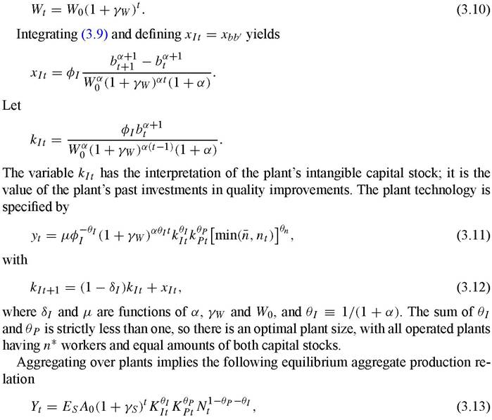
Following Parente and Prescott (2000), let the output of a quality b plant be given by the following equation,

¹⁷ For example, Schmitz (2001) suggests a mapping from government subsidies directed at state-owned en­terprises to aggregate efficiency.

¹⁸ See Parente and Prescott (2000) for a survey of this evidence.

With this technology, a minimum number of workers, n, is required to operate a plant. The variable k_P denotes the physical capital input. The subscript P is introduced in order to differentiate physical capital from intangible capital later in the analysis. There are no increasing returns to scale in the economy, because if the inputs of the economy are doubled, the number of plants doubles.¹⁹

A plant’s quality is a choice variable. To improve its quality, resources are needed. This resource cost is the product of two components. The first component is technolog­ical in nature and reflects the cost in the absence of constraints. The second component, denoted by φj > 1, reflects the constraint itself. The function that gives the required resources a plant must expend to advance its quality from b to b' is

Here W_t is the stock of pure knowledge in the world in period t. Its growth rate is exogenous and equal to γ_w. Thus

^[1] See Hornstein and Prescott (1993) for a detailed coverage of this technology.

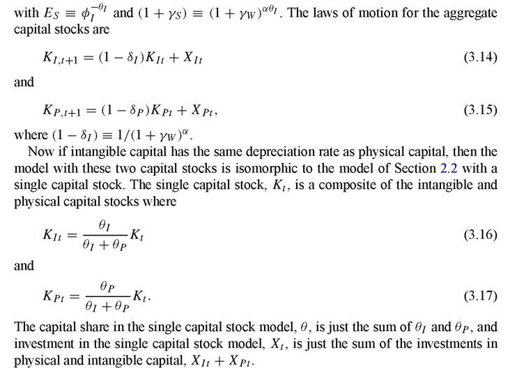
For the sake of consistency and brevity, we continue to use the model economy with a single capital stock in our presentation of the unified theory of the evolution of inter­national incomes. In those instances where we wish to consider the role of intangible capital, we proceed by assigning a value to the capital share parameter in the modern production function that exceeds 0.40, the share of physical capital’s output in the na­tional income accounts. We solve out the model economy with a single capital stock and then impute the intangible and physical capital components, as well as their investments. This can effectively be done using Equations (3.16) and (3.17) given a decomposition of the total capital share into its intangible and physical components.^[262]

3.3. Estimates of aggregate relative efficiency

The mappings developed in the preceding subsection allow us to impute the aggregate relative efficiency associated with the modern production function for various con­straints. In general, the size of the effect of the constraint on a country’s aggregate

efficiency depends on the factor input affected by the constraint and on that input’s share in the production function. In the special case where the constraints affect all in­puts equally, that is, φ = φ_n = φj = φ_p,the individual factor shares are unimportant and the efficiency level of a country is just E_s = φ~^l. Hence, the implied difference in relative efficiencies is equal to the implied cost differences of policy. Thus, if the cost difference in policies between two countries is a factor of five, the implied factor difference in aggregate relative efficiency is also five.

Are factor differences in relative efficiency greater than five reasonable? Obviously, it is not possible to answer this question definitively without a comprehensive interna­tional study of the total costs of the constraints imposed by society. Some estimates of the cost differences associated with some country-specific policies do exist. Studies that estimate the costs of certain policies of individual countries that affect the technology and work practice choices of the production units located there do find that these costs vary systematically with income levels, with large differences existing between rich and poor countries. These studies suggest that factor differences in relative efficiencies could easily be as great as five.

For example, Djankov et al. (2002) calculate the costs associated with the legal re­quirements in 75 countries that an entrepreneur must meet in order to start a business. They find that the number of procedures required to start up a firm varies from a low of 2 in Canada to a high of 20 in Bolivia and that the minimum official time required to complete these procedures ranges from a low of 2 days in Canada to a high of 174 days in Mozambique. These costs do not reflect any unofficial costs involved with starting a firm, such as bribes or bureaucratic delays. Because these official cost measures are pos­itively correlated with indexes that incorporate measures of bribes, the true difference in start-up costs between low-cost and high-cost countries is surely even larger than those reported in the study.

3.4. Reasons for constraints

The evidence strongly suggests that production units in poor countries are severely con­strained in their choices, and the costs associated with these constraints are large. This prompts the question: Why does a society impose these constraints? A large number of studies, some of which are surveyed in Parente and Prescott (2000), suggest that constraints typically are imposed on firms in order to protect the interests of factor suppliers to the current production process. These groups stand to lose in the form of reduced earnings if new technology is introduced. These losses occur because either the input they supply is specialized with respect to the current production process or their industry’s demand is price inelastic.^[263]

4.