A theory of economic development
In this section, we present the theory of economic development put forth by Hansen and Prescott (2002). We do this in three stages. First, we describe the classical component of that theory and derive its equilibrium properties.
Next, we describe the modern growth component of that theory, and also derive its equilibrium properties. The last stage merges these two components and, in doing so, presents the Hansen and Prescott model of economic development.Figure 2 describes the general pattern of economic development. More specifically, Figure 2 reports per capita income of the leader country dating back to 2000 B.C. Up until 1700, the living standard in the leader country, or any other country for that matter, displayed no secular increase. These living standards were significantly above the subsistence level. In 1688, for example, the poorest quarter of the population in England - the paupers and the cottagers - survived on a consumption level that was roughly
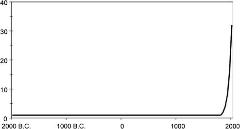
Figure 2. Income per capita of the leader relative to the pre-1800 level. Source: Bairoch (1993).
one-fourth the national average.[250] A few societies, such as the Roman Empire in the first century, the Arab Caliphates in the tenth century, China in the eleventh century, and India in the seventeenth century, realized some increases in their per capita income. However, these increases were not sustained. After 1700 per capita income in England started to increase. Over the next 150 years, these increases in the leader country were modest and irregular. However, since 1900, these increases have been larger and fairly regular, with per capita income doubling roughly every 35 years.
Technology was not stagnant over any part of this time period. Economic historians have documented a steady flow of technological innovations in this 2000 B.C.
to A.D. 1700 period.[251] Yet these innovations prior to 1700 did not translate into increased living standards. Instead they translated into increased population: as total output increased, the population adjusted so as to maintain a constant level of per capita output. After 1700, these innovations did translate into increases in living standards.2.1. Classical theory: the pre-1700 era
Classical economists, most notably Malthus and Ricardo, devised a theory that accounts well for the constant level of per capita income that characterized the pre-1700 era. The theory predicts a trade-off between living standards and population size. This trade-off exists because population growth is an increasing function of per capita consumption and because there is an important fixed factor of production, namely, land. A key implication of this theory is that there is a constant standard of living to which the economy adjusts. The theory predicts that increases in the stock of usable knowledge, which could translate into increases in living standards, instead translate into increases in population.
Malthus' theory of population is a biological one rather than an economic one. According to his theory, fertility rises and mortality falls as consumption increases. Being classical, the model has no utility theory and so agents have no decision over the number of children they have. Recently a number of authors, including Tamura (1988), Becker, Murphy and Tamura (1990), Doepke (2000), Galor and Weil (2000) and Lucas (2002), have generated Malthus-like population dynamics in a neoclassical model with household utility defined over consumption of goods and number of children. These models follow Becker (1960) by having a trade-off between quality and quantity of children.
We do not take their approach in this chapter. Instead the approach we take has society through its institutions and policies implicitly determine its population size. Although we similarly add household preferences to the classical theory of production, we do not define household preferences to be over the quantity of household children.
Consequently, in this societal theory of population growth, the quantity of children is treated as exogenous from the standpoint of the household.The reason we take this societal approach to population growth is twofold. First, there is no tested theory of population dynamics, and once modern economic growth begins, demographics play a secondary role in development. Second, and more important, the approach reflects the view that groups of individuals, namely, societies, have had a much larger say in deciding how many children a family has than the family itself. Societies have instituted and continue to institute policies that give them their desired population size. Often the policies of society are not what individual families want. In modern China, for example, a law effectively limits many households to one child. By contrast, Iran in the 1980s wanted a higher population and so implemented subsidies to encourage people to have more children. After achieving its objective, the government stopped these subsidies in the 1990s and began to subsidize contraceptives. India today, wanting a lower population growth rate, has set up family planning programs in many regions. In all these cases, the effects of policy upon demographics are dramatic. Even in poor and rural Indianvillages, which did not experience any increase in human capital or income, policy has led to a dramatic decline in population growth rates in the late twentieth century.
Why did society choose population size prior to 1700 so as to maintain a constant living standard? The answer relates to the fact that land was an essential input to the production process in the pre-1700 era. In particular, as a valuable resource, land was subject to expropriation by outsiders. Prior to 1700, a small group of people with large amounts of quality-adjusted land and therefore a high living standard could not defend this land from outside expropriators. For this reason, there was a maximal sustainable living standard.
Society set up social institutions that controlled population so as to maintain the highest possible living standard consistent with the ability to defend itself from outside expropriators. Once an economy switches to the modern production technology, land is no longer an important input, so its defense is not an issue. At the stage when the modern production technology dominates, society sets up its social institutions that it sees as maximizing living standards subject to a constraint that a society perpetuates itself.For the purpose at hand, it is not essential that we model society’s choices of institutions that affect fertility choices. Instead, it is sufficient to treat the growth rate of population in a simple mechanical way, namely, as a function of average consumption. In order to reflect society’s choices, the function must display two properties. First, it must have a large positive slope, in the neighborhood of the pre-1700 consumption level. Second, for high levels of average consumption, the slope of the function must be near zero. The first property is only relevant for the theory of the pre-1700 era. The second property is only relevant for the theory of the post-1900 period. This is the approach that we take in this essay.
With this in mind, we proceed with a neoclassical formulation of the classical theory of constant living standards. There is a single good in the model that can be used for either consumption or investment purposes. The good is produced using a constant returns to scale technology that uses capital, labor, and land. An infinitely lived household owns the economy’s land and capital and rents them to firms in the economy. Land is fixed and does not depreciate. The household is made up of many members, each of whom is endowed with one unit of time. The household uses its capital, labor, and land income for consumption and investment purposes. The growth rate of population is a function of average consumption of household members.
A household member’s utility in the period is defined over the member’s consumption in the period. The household’s objective is to maximize the sum of each member’s utility. The details of the economy are described as follows.2.1.1. Technology
The classical theory of production is given by a Cobb-Douglas technology,
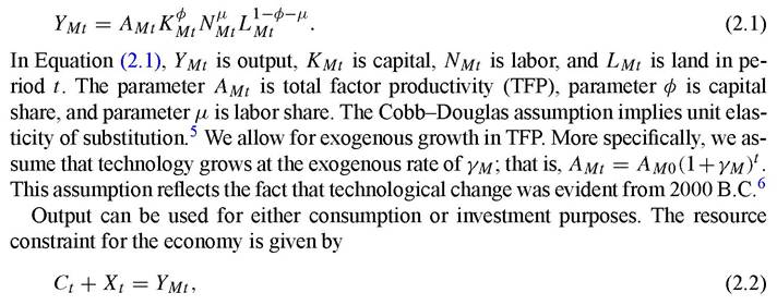
5 The precise value of the elasticity of substitution between land and the other factors is not important provided that it is not greater than one. The evidence is that throughout most of history the substitution of these other factors for land was limited and, if anything, this elasticity of substitution was less than one. The unit elasticity assumption is made because it simplifies the analysis.
6 We follow Hansen and Prescott’s convention of using the letter M to index variables associated with the classical production function.
where Ct denotes total consumption and Xt denotes total investment.
2.1.2. Preferences
Household preferences are added to the classical theory of production as follows. Period utility of each household member is defined over the member’s consumption of the final good. We assume a log utility function, because it is in the class of utility functions that is consistent with a constant-growth equilibrium and because empirically it is consistent with a wide variety of micro and macro observations. Household utility in each period is the sum of each individual member’s utility in the period. Strict concavity of individual household members’ preferences implies that the household’s utility is maximized by giving equal consumption to each member. For this reason, the discounted stream of utility of the household is just

where β is the time discount factor, ct is consumption of a household member, and Nt is household size.
As is evident from Equation (2.3), we are using a dynastic construct. This is in contrast to Hansen and Prescott (2002), who use a two-period overlapping generations construct. We adopt an infinitely lived household framework rather than the two-period overlapping generations framework for two reasons. First and foremost, the empirical counterpart of a period is a year in the dynamic construct, while in the two-period overlapping generations construct the empirical counterpart of a period is 35 years. For the purpose of examining the model’s ability to account for the large increases in output realized in a short period of time after 1950 by countries such as Japan and South Korea, 35 years is simply too long a period to study.
Second, the size of the effect on a country’s steady state level of per capita output associated with policies that determine its savings rate is sensitive to the construct that is used. The tax rate system of a country is an example of such a policy. The level effects associated with this type of policy are in fact larger with the dynastic construct. This fact is important for judging whether differences in savings rates can account for the large differences in transition dates. If plausible differences in savings rates fail to give rise to 200-year delays in development in the dynastic construct, then they also fail to give rise to this delay in the overlapping generations framework, and we can conclude that some factor other than savings rates accounts for the pattern of development.[252] This is essentially the finding of the quantitative exercises undertaken by Parente and Prescott (2000). The choice of construct is irrelevant, however, in assessing the plausibility of other factors such as efficiency, as reflected in TFP differences: the size of the level effects is the same regardless of whether the dynastic or overlapping generations construct is employed.
2.1.3. Endowments
Each member of the household is endowed with one unit of time, which the member can supply to firms in the economy to earn wage income. The household is also endowed with the economy’s stock of land and capital, which the household rents to firms. Land in the economy is fixed in supply: it cannot be produced, and it does not depreciate. Without loss of generality, the total quantity of land in the economy is normalized to one. Since land has no alternative use aside from production, the input to production in each period is one. Capital is assumed to depreciate and evolves according to the following law of motion

where δ is the depreciation rate.
2.1.4. Population dynamics
As mentioned earlier, because we take a societal approach to population size, we model population growth as a function of the average consumption level of household members. More specifically, we assume that the number of members born into a household in period t + 1 depends on the average consumption level of household members from period t. Let Nt denote the number of household members in period t, and let ct denote their average consumption level. Then

The function g is the growth factor of population from one period to the next. The classical prediction of a stable living standard at the pre-1700 level, cM, requires that the function g have a sufficiently large and positive slope at cM. This cM is the maximal living standard consistent with a society being able to defend its land.
2.1.5. Equilibrium properties
standard to rise above cM, say, because of plague or drought, population increase would exceed technological advances and the living standard would then fall until it returned to cM. If for some reason c were below cM, the population growth factor would be less than the one needed to maintain the living standard, and the living standard would increase until it was again cM. Along the steady-state equilibrium path, aggregate output, capital, consumption, and the rental rate of land all grow at the rate of the population. Per capita variables as well as the rental price of labor and capital are all constant. Increases in technology in this model simply translate into a higher population rather than a higher living standard. This is precisely the pattern of development observed prior to 1700.
2.2. Modern growth theory: the post-1900 era
The classical theory accounts well for the pattern of economic development up to 1700. However, it does not account for the increase in living standards that occurred after 1900. Since about 1900, the growth rate of the early developers has been roughly constant, with a doubling of per capita output every 35 years. Modern growth theory, in contrast, does account for the increase. In addition to the roughly constant rate of growth achieved by developed countries over the last century and a half, other facts characterize modern economic growth. These facts are roughly that the consumption and investment shares of output are constant, the share of income paid to capital is constant, the capital- to-output ratio is constant, and the real return to capital is constant.
Modern growth theory accounts well for these modern growth facts. Quantitatively, the steady-state equilibrium of the economy mimics the long-run observations of the United Kingdom and the United States. This is no surprise: Solow (1970) developed the theory with these facts in mind. A key feature of that theory is a Cobb-Douglas production function that includes no fixed factor of production and that is subject to constant exogenous technological change. More specifically, the production technology for the composite good that can be used for either consumption or investment purposes is given by
 ) In Equation (2.6), Yst is output, Kst is capital, and Nst is labor in period t. The parameter θ is capital share, and the parameter Ast is TFP, which grows exogenously at the constant, geometric rate γs. As can be seen, the critical difference between the traditional and modern growth production functions is that the modern growth function does not include the fixed factor input, land.[253]
Because the final objective of this section is to merge the classical theory and the modern growth theory into a single model, we maintain the same assumptions regarding preferences, endowments, and population dynamics as in the preceding subsection. The household in the model rents capital to firms and supplies labor. It uses its capital and labor income to buy consumption for household members and to augment the household’s stock of capital.
In contrast to the classical theory, population growth in the modern theory does not have any consequences for the growth rate of per capita variables in the long run. The choice of the population growth function is therefore unimportant in this respect. The standard procedure is to assume a population growth function g(c) that is constant over the range of sufficiently high living standards associated with the modern growth era. Population thus grows at a constant exponential rate.
Clearly, population cannot grow at an exponential rate forever. At some population level, natural resources would become a constraining factor. If population were ever to
reach this level, it would be unreasonable to abstract from land as a factor of production. But societies control their population so that it never reaches this level. Indeed, reproduction rates have fallen dramatically in the last 50 years, so much in the rich countries, in fact, that these countries must increase their fertility rates to maintain their population size in the long run. This suggests a population growth function that asymptotically approaches one.
In the case where the population growth function is a constant, per capita output, consumption, and capital all increase at the rate (1 + y⅛)1^1-^ along the equilibrium constant growth path. The rental price of labor also grows at this rate. The rental price of capital, in contrast, is constant. Consumption’s share and investment’s share of output are also constant as is capital’s share which is equal to θ. As can be seen, the growth rate of the economy’s living standard is independent of the economy’s population growth rate: the only thing that matters is the exogenous growth rate of technological change. The population growth rate does have an effect on the level of per capita output along the constant growth path, but it is small. Thus, unlike in the model of the pre-1700 era, the population growth function in the model of the post-1900 era plays only a minor role.
2.3. The combined theory
The classical theory accounts well for the constant living standard that characterizes the pre-1700 era, and the modern growth theory accounts well for the doubling of living standards every 35 years that characterizes the post-1900 experience of most of the currently rich, large, industrialized countries. In the period in between, living standards increased in these countries, but at a slower and far more irregular rate compared to the post-1900 period.
We seek a theory of this development process, namely, a theory that generates a long period of stagnant living standards up to 1700, followed by a long transition, followed by modern economic growth. Given the success of the classical theory and the modern growth theory in accounting for the pre-1700 and post-1900 eras, the logical step, and the one taken by Hansen and Prescott (2002), is to merge the two theories by permitting both technologies to be used in both periods. We now present the combined theory of Hansen and Prescott, and use that theory to organize and interpret the development path of the leading industrialized country over the 1700-2000 period.
In the combined theory of Hansen and Prescott (2002), output in any period can be produced using the traditional or the modern growth production function or both. Both technologies, therefore, are available for firms to use in all periods.[254] Capital and labor are not specific to either production function. In light of these assumptions, the aggregate resource constraint for the combined model economy is

the capital rental market-clearing constraint is

and the labor market-clearing condition is

Household preferences continue to be given by Equation (2.3). Additionally, the population growth function continues to be given by Equation (2.5), and it displays the properties that the function has a large positive slope in the neighborhood of the pre-1700 consumption level and a slope near zero for large levels of consumption.
In their combined theory, Hansen and Prescott assume that the growth rate of TFP for the traditional production function and the growth rate of TFP for the modern economic growth production function are each constant over time. We deviate from Hansen and Prescott on this dimension. Although we maintain their assumption that the rate of TFP growth associated with the traditional technology is constant, we assume that the rate of TFP growth associated with the modern growth technology increases over time, converging asymptotically to the modern growth rate. We make this alternative assumption in light of the empirical counterparts of the two production functions and the historical evidence on technological change.
The empirical counterpart of the classical production function is a traditional technology for producing goods and services that is most commonly associated with the family farm. A key feature of this production technology is that it is based on the use of land in the production of hand tools and organic energy sources. For this technology, the historical record shows gradual improvements in these methods over the last 2,000 years at a roughly constant rate of change.[255] [256] The empirical counterpart of the modern growth production function is a modern technology that is most commonly associated with the factory.11 A key feature of this technology is that it uses machines driven by inanimate sources of energy. For this technology, the historical record suggests modest growth in the eighteenth century, followed by much higher growth in the nineteenth and twentieth centuries. Lighting, communication, and transportation were important areas where this accelerating pattern occurred. Consequently, a more plausible assumption is that the growth of TFP associated with the modern production function increased slowly after 1700 and converged to the rate associated with the modern growth era shortly after 1900.
We emphasize that the traditional sector should not be thought of as primarily the agricultural sector, though most outputs of this sector are agricultural products. What characterizes the traditional sector is that the household is the producing unit and typically consumes much of what it produces. Sugar plantations in the Caribbean and cotton plantations in the United States were not part of the traditional sector. There was little incentive for people working in the traditional sector to develop more efficient production methods. Rapid increases in agricultural productivity occurred only when goods developed in the industrial sector were introduced in farming. The reaper and the tractor dramatically increased productivity on farms. Insecticides and fertilizers also contributed to productivity, as did the development of hybrid corn and new seeds. This is all well documented by Johnson (2000).
An economy that starts out using only the traditional production function will eventually use the modern one. To see this, suppose that it were never profitable for firms to use the modern production function. Then the economy’s equilibrium path would converge to the steady state of the pre-1700-only model. The steady state of that model is characterized by constant rental prices for capital and labor, rM and wM. Capital and labor are not specific to any one technology. Thus, a firm that first considers using the modern production function can hire any amount of capital and labor at the factor rental prices rMt and wMt. Profit maximization implies that a firm will not choose to operate the modern growth technology if

This inequality must be violated at some date. Asymptotically, the rental prices would approach constant values if only the traditional production function were operated, and so the right-hand side of (2.10) is bounded. The left-hand side is unbounded because TFP in the modern function grows forever at a rate bounded uniformly away from zero. The inequality given by (2.10), therefore, must eventually be violated.
At the date when TFP in the modern production function surpasses the critical level given by the right-hand side of (2.10), the economy will start using the modern growth production function. This marks the beginning of the Industrial Revolution. This result is independent of the size differences in the growth rates of TFP associated with the traditional and modern production functions. Over the transition, more and more capital and labor will be moved to the modern production sector. The traditional production function will, however, continue to be operated, though its share of output will decline to zero over time. This follows from the assumptions that land is used only in traditional production and that its supply is inelastic.
We now use the combined theory to organize and interpret the development path of the industrial leader over the 1700-2000 period. The empirical counterpart of a period is a year. The initial period of the model is identified with the year 1675.[257] We attribute the stagnation of the leader prior to 1700 to an insufficiently low level of TFP associated with the modern production function to warrant its use. We attribute the start of economic growth of the leader in 1700 to growth in TFP associated with the modern production function so that its level exceeds the critical value given by Equation (2.10). Lastly, we attribute the rising rate of growth of per capita output of the leader from 1700 to 1900 to greater use of the modern production function and the rising rate of growth of TFP.
We proceed to parameterize the model. The model is calibrated so that the economy starts to use the modern production function in 1700. Following Hansen and Prescott (2002), we calibrate the model so that the steady state of the classical-only model (Section 2.1) matches pre-1700 observations and the steady state of the modern growth-only model (Section 2.2) matches the post-1900 growth experience of the United States.
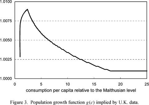
In the calibration, we deviate from Hansen and Prescott along two dimensions. First, we calibrate the population growth function so that it matches Maddison’s (1995) estimates for U.K. population growth rates over subperiods of the 1675-1990 period.[258] Given our theory of population growth, it is more appropriate to use the time series data from a particular country to restrict the population growth function for that country rather than cross-section data as Hansen and Prescott do.[259] Second, we calibrate the annual growth rate of TFP for the modern production function so that it remains at the traditional rate up until 1700, increases linearly to reach one-half of its modern growth rate in 1825, and then increases linearly to reach its modern growth rate in 1925.
Following Hansen and Prescott, we pick the initial capital stock and the initial population so that if only the traditional production function were available, the equilibrium would correspond to the steady state of the pre-1700 model, and there would be no incentive to operate the modern production function if it were available. This ensures that in period 0 only the traditional production function is operated and that there is a period of constant living standards. Table 1 lists the values for each of the model parameters and provides comments where appropriate. The population growth rate function implied by the U.K. population growth data used in the computation is depicted in Figure 3.
For the parameterized model economy, it takes 150 years before 95 percent of the economy’s output is produced in the modern sector. Figures 4-6 depict the model economy’s development path along a number of dimensions. Figure 4 compares period t per capita output relative to 1700 per capita output for the model economy and the industrial leader as reported by Maddison (1995, Tables 1.1 and C.12). According to the model, an economy that begins the transition in 1700 will be approximately 28 times richer in
Table 1
Restricted parameter values
| Parameter | Value | Comment |
| YM - growth rate of TFP for | 0.0009 | Consistent with pre-1700 world population |
| traditional production | average annual growth rate of 0.003 | |
| φ - capital share in | 0.10 | Consistent with pre-1700 estimates of |
| traditional production | land’s share reported by Clark (1998) and Hoffman (1996) | |
| μ - labor share in traditional | 0.60 | Chosen so that labor’s share does not vary |
| production | with the level of development as reported by Gollin (2002) | |
| Am0 - initial TFP for | 1.0 | Normalization |
| traditional production | ||
| δ - depreciation rate | 0.06 | Consistent with U.S. capital stock and investment rate since 1900 |
| YS - asymptotic TFP growth | 0.012 | 2 percent rate of growth of per capita GDP |
| rate for modern production | in modern growth era | |
| θ - capital’s share in modern | 0.40 | U.S. physical capital’s share of output |
| production | ||
| As0 - initial TFP for modern | 0.53 | 1700 starting date given initial period for |
| production | model is 1675 | |
| β - subjective time discount | 0.97 | Consistent with real rate of interest between |
| factor | 4 and 5 percent in modern growth era | |
1990 than in 1700. Figure 5 depicts the growth rate of per capita output for the model economy over the 1700-2000 period. The growth rate of per capita output is slow at the onset of the transition, less than 1 percent per year on average before 1825. By 1900 the growth rate is near the modern growth rate of 2 percent per year. This pattern is
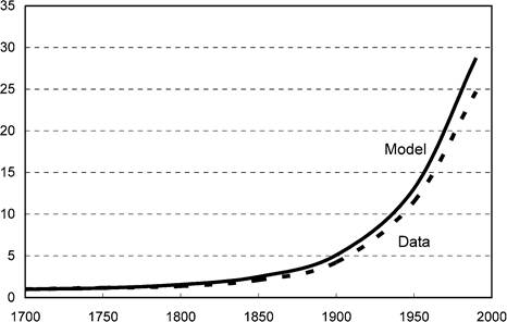
Figure 4. Income per capita relative to 1700. Source: Maddison (1995).
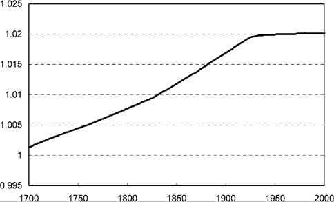
Figure 5. Predicted growth rate of per capita output, 1700-2000.
primarily a consequence of the assumption that TFP growth for the modern technology increases slowly over the 1700-1900 period. Figure 6 depicts the path of the rental prices of capital and labor over the 1700-2000 period. As can be seen, the real wage rate increases steadily once the transition begins. The real interest rate, in contrast, shows very little secular change over three centuries. These latter predictions conform well to the pattern of development associated with England, the United States, and other early developers.
The predictions of the model are not sensitive to the value of the capital share parameter in the modern growth production function. This is an important result, because the magnitude of the capital share with a broad definition of capital that includes intangible as well as tangible capital could well be greater than the 0.40 share value used in the above exercise. The paths of per capita GDP, its growth rate, and rental prices are
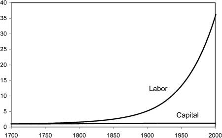
Figure 6. Predicted factor rental prices (1700 = 1), 1700-2000.
nearly identical to those shown in Figures 4-6 for alternative values of the capital share in the modern production function. The transition still takes a long time. For a capital share as high as 0.70, 140 years elapse before 95 percent of the economy's output is produced using the modern production function.
3.
More on the topic A theory of economic development:
- Conclusion
- Background Context
- BACKGROUND AND DEFINITIONS
- INTRODUCTION
- Oman
- THE BIG DATA ECOSYSTEM
- Introduction
- Malta
- Risks and sources of policy failure
- Qatar