Urbanization and growth

The previous section examined a fully urbanized economy where all production occurs in cities. City sizes grow with improvements in technology; but, absent stochastic el­ements, individual cities grow in parallel, with the relative numbers of different types of cities and the relative size distribution of cities time invariant.

3.1. Two sector approaches, without cities

Urbanization involves resources shifting from an agricultural to an urban sector. The dual economy models dating back to Lewis (1954) look at sectoral change but are really static models. They focus on the question of urban “ bias”, or the effect of government policies on the urban-rural divide, and the efficient rural-urban allocation of population at a point in time. These two sector models have an exogenously given “sophisticated” urban sector and a “backward” rural sector [Rannis and Fei (1961), Harris and Todaro (1970), and others] as now well exposited in textbooks [e.g., Ray (1998)].

In these models, the marginal product of labor in the urban sector is assumed to exceed that in the rural sector. Arbitrage in terms of labor migration is limited by inef­ficient (and exogenously given) labor allocation rules such as farm workers being paid average rather than marginal product or artificially limited absorption in the urban sector (e.g., formal sector minimum wages). The literature focuses on the effect on migration from the rural to urban sector of policies such as rural-urban terms of trade, migration restrictions, wage subsidies, and the like.

The final and most complex versions of dual sector models are in Kelly and Williamson (1984) and Becker, Mills and Williamson (1992), which are fully dynamic CGE models. They have savings behavior and capital accumulation, population growth, and multiple economic sectors in the urban and rural regions. Labor markets within sec­tor and across regions are allowed to clear. The models analyze the effects of a wider array of policy instruments, including sector specific trade or capital market policies for housing, industry, services and the like. However the starting point is again an ex­ogenously given initial urban-rural productivity gap, sustained initially by migration costs and exogenous skill acquisition. On-going urbanization is the result of exogenous forces - technological change favoring the urban sector or changes in the terms of trade favoring the urban sector.

As models of urbanization, these dual economy ones are a critical step but they suf­fer obvious defects. First how the dual starting point arises is never modeled. Second, and related to the first, there are no forces for agglomeration that would naturally fos­ter industrial concentration in the urban sector. Finally although the models have two sectors there is really little spatial or regional aspect to the problem. There is a new generation of two-sector models, the core-periphery models, which attempt to address some of these defects. The core-periphery models ask under what conditions in a two- region country, industrialization, or “urbanization” is spread over both regions versus concentrated in just one region.

Comparedto the dual economy models, Krugman’s (1991a) paper explicitly has scale economies that foster endogenous regional concentration. Second, while there are two regions, no starting point is imposed, where one region is assumed to start off ahead of the other. Industrialization may occur in both regions or in only one region. One region can become “backward” (under certain assumptions), or, if not backward (lower real incomes) at least relatively depopulated [Puga (1999)].

The models are focused on a key developmental issue - the initial development of a core (say, coastal) region and a periphery (say, hinterland) region, as technology im­proves (transport costs fall) from a situation starting with two identical regions. As such they do relate to the earlier discussion in Section 1.3 of urban concentration in a primate city versus the rest of the urban sector. Some work [Puga (1999), Fujita, Krugman and Venables (1999, chapter 7), Helpman (1998) and Tabuchi (1998)] also analyzes how under certain conditions, with further technological improvements, there can be reversal. Some industrial resources leave the core; and the periphery also in­dustrializes/urbanizes. However core-periphery models have limited implications for urbanization per se, since in many versions including Krugman (1991a) initial paper, the agricultural population is fixed.

Unfortunately, to date core-periphery models have been almost exclusively uni­dimensional in focus, asking what happens to core-periphery development as transport costs between regions decline. They are not focused on other forms of technological advance, let alone endogenous technological development. With a few exceptions such as Fujita and Thisse (2002) and Baldwin (2001), the models are static. But even in these exceptions, there is still the focus on exogenous changes in transport technology. Compared to the older dual economy literature, generally core-periphery models have no policy considerations of interest to development economists, such as the impact of wage subsidies, rural-urban terms of trade, capital market imperfections. An exception is that some papers have examined the impact on core-periphery structures of reducing barriers to international trade, such as tariff reduction; and papers are starting to explore issues of capital market imperfections.

The dual economy and core-periphery models are regional models, with limited ur­ban implications. Urban models are focused on the city formation process, where the urban sector is composed of numerous cities, endogenous in number and size. Efficient urbanization and growth require timely formation of cities. As policy issues the extent of market completeness in the national markets in which cities form, the role of city governments and developers, the role of inter-city competition, and the role of debt fi­nance and taxation are critical. In the next section we analyze an urbanization process in which there are cities. Then we turn to a discussion of some key policy issues.

3.2. Urbanization with cities

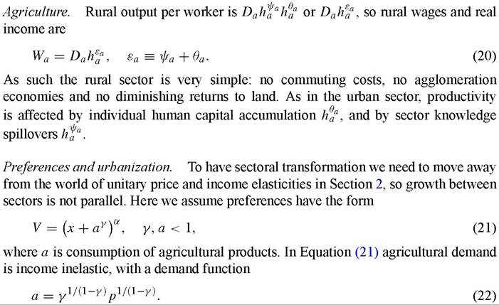
Here I present a simple two sector model of urbanization with cities, adapting the model in Section 2 following Henderson and Wang (2005a, 2005b). The urban sector is ex­actly like the X₁ city sector earlier, with production technology given in (6). The other sector is food produced in the agriculture sector, which we make now the numeraire (since there may initially be no urban sector). As a result, for type 1 cities in the urban sector, Equation (7) for wages, Equations (9) and (10) for commuting costs and rents, and Equation (15) for income are all redefined to be multiplied by the price of X₁, p. The city size equation is the same, invariant to relative prices. Critical here is for Q₁ a parameter cluster.

3.2.1.

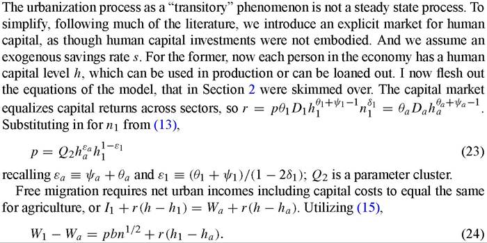
With free migration equalizing real incomes across sectors, urban wages exceed rural wages by (commuting) cost-of-living differences [the first term on the right-hand side of (24)], and by a factor compensating if human capital requirements in the urban sector exceed those in the rural, as I assume.

If we substitute in (24) for W₁, W_a, p and r and rearrange, we get

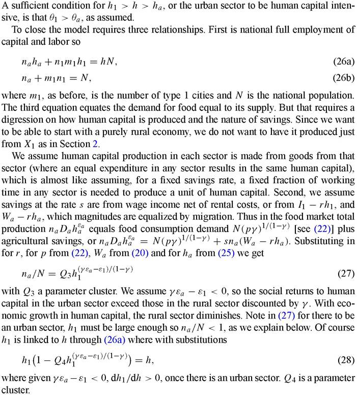
3.2.2. Urban growth and transformation

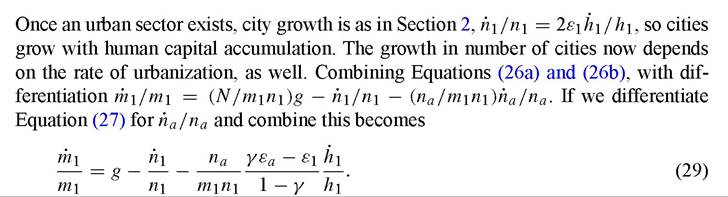
As before, the rate of growth of numbers of cities is increased by national population growth, g, and reduced by growth in individual city sizes. Now it is also enhanced by economic growth which increases relative demand for urban products and draws labor out of agriculture, as captured by the last term in Equation (29).

3.2.3. Economic growth

3.3. Extensions and policy issues

There are three general sets of policy issues. First concerns whether in the context of the models in Sections 2 and 3.2, the national composition of cities of different types is efficient. We have already discussed this issue: in many contexts asking whether the national composition of cities is efficient is the same as asking if national output composition is efficient. If there are national policy biases such as trade policies favor­ing steel products over textile products, with urban specialization, if steel is produced in bigger types of cities than textiles, the numbers of larger cities relative to smaller ones and hence urban concentration will increase.

The second general set of issues deals with factors we have ignored. In particular, the modeling in Sections 2 and 3.2 assumes a nice smooth process where (i) all factors of production are perfectly mobile and malleable, (ii) city borrowing and debt accu­mulation have no role, (iii) “lumpiness” problems that arise in city formation when economies are small are ignored: while m must be an integer in reality, in the analysis it is treated as any positive number where the number of cities grows at a rate m/m, rather

than by 0, 1 or 2. A model that incorporates these features is outlined in Section 3.3.2, which brings to the forefront a variety of policy issues.

3.1.1. City sizes

A perpetual debate in particular developing countries is whether certain megacities are oversized, squandering national resources that must be allocated to commuting, congestion, and transport in those cities and resulting in low quality of life in the pol­luted, unsanitary and crowded slums of such cities. In other countries, especially former planned economies, the debate goes the other way: are cities too small? The growth con­nection is straightforward. Either squandered resources in over-sized cities or too small cities with unexploited scale economies mean lower income levels, potentially lower savings, lower capital accumulation and thus lower growth rates. While calculations are tedious, in the steady state growth in Section 2.2.2 where γ^h = h/h = (A - ρ)∕σ, A depends on urban parameters (for example, increasing with human capital returns) and will be lowered if city sizes are inefficient.

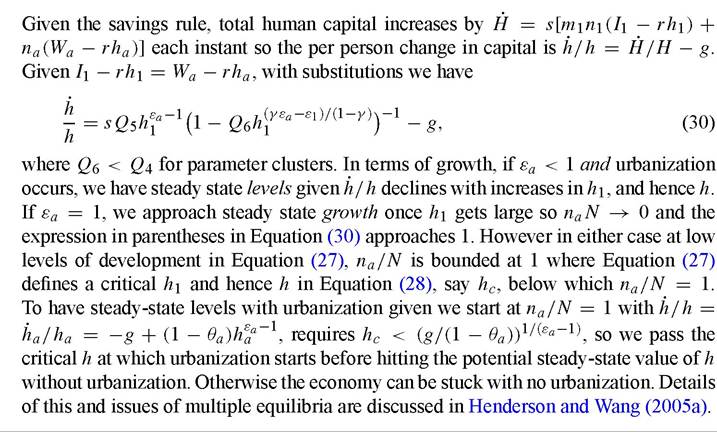
Using a simple, partial equilibrium diagram, it is possible to illustrate both issues: the megacity “problem” and the planned economy problem. The diagrams point to first- order effects. Forthe megacity problem, suppose there are a variety of type 1 cities in an economy with free mobility of labor and institutions supporting efficient city formation. In Figure 5(a), the representative city has a size n*, where real income as function of city size peaks at I₁*, tangent to the perfectly elastic national supply curve of labor to the city, given perfect labor mobility. Suppose one particular type 1 city is favored relative to the rest, where various types of favoritism are discussed in Section 1.3.2. For example it may have special public services compared to other cities financed out of national taxes. Those favors raise the realized utility, or real income that residents in the favored city potentially receive, shifting up the inverted-U real income curve. That upward shift draws migrants into the city expanding its size to n_mega. But at n_mega, the net income generated by the city, ignoring its nationally financed favors, is only net I_m. The gap, I* — I_m, times the population represents “squandered resources”. Of course, such squandering would in general equilibrium affect prices, lowering the height of the population supply curve and the inverted-U’s.

A second issue in city formation concerns poor institutions in national land markets and in local governance which limit the number of cities that can form. Suppose that, in villages which might become cities, local governments by institutional restrictions cannot expand infrastructure (see the next section), cannot rezone and build on urban fringe land, and cannot offer subsidies to incoming firms. And suppose developers can­not assemble large tracts of land for development because property rights are ill-defined. These villages cannot grow into cities; as well, entirely new cities cannot form. If the number of cities is bindingly limited, so there are too few cities, all existing cities under free migration are too big. In Figure 5(a), suppose we reconsider the figure ignoring the representative city curve and assume all cities have inverted-U’s like the favored city. Then, in this reinterpretation of the figure, I_f is the potentially attainable real income

(a)

(b)

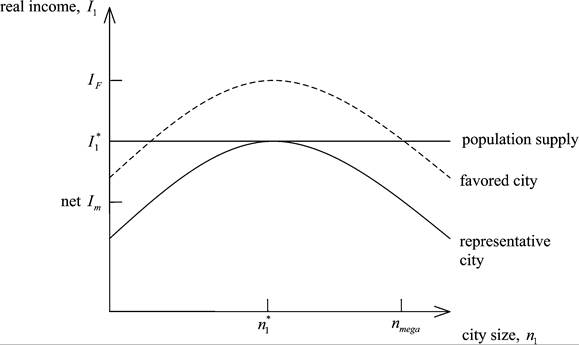
Figure 5. City sizes. (a) Favored cities. (b) Migration restrictions.

in all cities (ignoring general equilibrium effects) if cities could freely form. Given re­stricted numbers, rather than operating at I_f (with size n*), cities are overcrowded; and in equilibrium they operate at, say I₁* (with size n_mega), with the same national supply curve of labor as labeled in the figure. The restrictions result in losses related to the gap I_f - I*.

The planned economy problem is entirely different. Former “planned” economies like China have formal migration restrictions limiting the visas given for rural peo­ple to move to cities and limiting migrants’ access to jobs, housing, medical care and schooling in destination cities to reduce the incentive to migrate. Some former planned economies (as well as China) limited migration through housing provision and land de­velopment. If the state provides and allocates all housing assignments, migrants cannot move unless housing is provided in the destination. As we saw in Table 2, countries like China and Russia have very low urban concentration compared to other large coun­tries. Figure 5(b) captures the essence of the problem. While the representative city has an inverted-U where real income is maximized at rif migration restrictions for cities a and b restrict sizes to n_a and n_b and real incomes to I_a and I_b. Au and Henderson (2005) estimate these inverted-U’s for different types of cities in China in 1997 and find that 30% of cities are significantly undersized - below the lower 95% confidence interval on their equivalent to n*. The productivity losses from being undersized are enormous: 30-50% or more loss in GDP per capita for many cities.

3.1.2. Sequential city formation and governance

In a working paper, Henderson and Venables (2005) take a new approach to city for­mation. They assume a context where (1) there is a steady-flow of migrants from rural to urban areas, and (2) urban residence requires a fixed investment in nonmalleable, immobile capital (housing, sewers, water mains, etc.). Cities form sequentially with­out population swings, so migrants all flow first into city 1 until its equilibrium size is reached (abstracting from any on-going technological change), and then all future mi­grants all go to a second city until its equilibrium size is reached, and so on. This is a very different process than when all resources are mobile. In the usual models in a small economy, when the second city forms, it takes half the population of the first at that in­stant, and when the third forms it takes one third of the then population of the first two. Cities grow way past nf shrink back to nf and then grow again, shrink, and on so. With fixed capital, such population swings would mean periods of abandoned housing. With sufficiently high required fixed capital investments, all population swings are eliminated in equilibrium. Each new city starts off tiny with no accumulated scale effects and low productivity. It grows steadily absorbing all new rural-urban migrants until its growth interval is complete and it reaches steady state size; then a new city starts off growing from a tiny size.

With sequential city formation without population swings, given discounting of the future, efficient city size requires cities to grow past the equivalent of n*_l to their steady­state size nopt, at which point real income per worker is declining. Intuitively, growing past rif with declining but still high real income, postpones the formation of a new city with tiny population, no scale effects and very low incomes. The paper then looks at equilibrium city formation in two contexts.

First is a situation with no “large agents” in national land markets - no developers and no city governments. In a model with perfect mobility of resources as discussed in Section 2, city formation with atomistic agents is a disaster due to coordination failure. A new city can only form when old cities are so big that the income levels they offer

have fallen to the point where they equal what a person can earn in a city of size one. Having immobile capital presents a commitment device [Helsley and Strange (1994)], so individual, sequentially rational builders switch from building in an old city to build­ing in a new one at a “reasonable time”. Real incomes are still equalized across cities through migration. Given big old cities have high nominal incomes and the tiny new one low nominal income, housing rents adjust in old cities to equalize real incomes. Hous­ing rents in old cities change over the growth cycle of a new city, starting very high and then declining [see also Glaeser and Gyourko (2005)]. In this context, equilibrium city sizes may even be smaller than optimal ones. The deviation from optimum has not to do with coordination failure which is solved despite the absence of “large” agents, but with the present value of externalities created by the marginal migrant in an old versus a new city.

With developers or full empowered local governments, externalities are appropri­ately internalized and city sizes are n_opt. However, apart from financing the housing and infrastructure capital, to induce new migrants to move to a new city with its low real in­come and scale economies in a timely fashion, governments must subsidize in-migration of worker-firms. To do this they must borrow and, in fact, public debt accumulates over the entire growth interval of a city and only starts to be paid off once it reaches steady­state size. Debt ceilings, or limits for cities which are common in many countries curtail subsidies to in-migrants and postpone new city formation. Debt limited cities are too big. The paper also explores the effects of limits on local tax property tax powers.

4.