Cities and growth

To establish the links between cities, growth, urbanization, urban concentration and policy, we look at models in which cities are a defined unit, endogenous in number and size. These are systems of cities models which date to Henderson (1974), with a variety of substantial contributors to further development [Hochman (1977), Kanemoto (1980), HendersonandIoannides (1981), Abdel-RahmanandFujita (1990), Helsley and Strange (1990), Duranton and Puga (2000) and Rossi-Hansberg and Wright (2004), to name a few].

2.1. The systems of cities at a point in time

Consider a large economy composed of two types of cities, where there are many cities of each type and each type is specialized in the production of a specific type of traded good. We will show why (when) there is specialization momentarily; the generalization to many types of goods and cities is straightforward. To simplify the growth story, each firm is composed of a single worker. In a city type 1, in any period, the output of firm i in a type 1 city is

where h_1i is the human capital of the worker and is his input in the production process.

In this section spatial decay is all or nothing - no decay within the city’s; 100% across cities. As such in (6), n₁ could represent the total volume of local spillover com­munications, where δ₁ is the elasticity of firm output with respect to n₁. The restriction δ₁ < 1/2 which limits the degree of scale economies ensures a unique solution in an economy composed of many type 1 cities. Without the restriction, all X₁ produc­tion crowds into just one city. Note the production process ignores land, collapsing the central business district (CBD) to a point. There is a recent literature building upon Fujita and Ogawa where firm density is endogenous in a spatial CDB with information spillover decay. There market equilibrium density is nonoptimal because firms in mak­ing location decisions do not recognize that choices leading to greater densities would enhance information spillovers [Lucas and Rossi-Hansberg (2002) and Rossi-Hansberg (2004)]. The issue of central city design and zoned density is an important one in the design of cities in developing countries.

The second externality in (6) derives from h₁, the average level of human capital in the city, which represents local knowledge spillovers. h^ψ could be thought of as the richness of information spillovers n^δ1¹, so that knowledge enhances (multiplies) local information spillovers, or gives better information. Alternatively it could just represent the level of local technology, which increases as average education increases locally.

Given this simple formulation the wage of worker i in city type 1 is

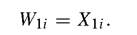(7)

In an economy of identical individual workers in type l cities, individuals will all have the same human capital level (either exogenously in a static context, or endogenously in a growth context). Thus total city output is

2.1.1. Equilibriumcitysizes

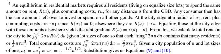
Equations (6) and (8) embody the scale benefits of increases in local employment, where output per worker is an increasing function of local own industry scale. Determinant city sizes arise because of scale diseconomies in city living, including per capita infrastruc­ture costs, pollution, accidents, crime, and commuting costs. In Henderson (1974) those are captured in a general cost of housing function, but most urban models consider an explicit internal spatial structure of cities. As noted all production occurs at a point, the CBD. Surrounding the CBD in equilibrium in local land markets is a circle of residents each on a lot of unit size. People commute back and forth at a constant cost per unit (return) distance of τ. That cost can be from working time, or here an out-of-pocket cost paid in units of X1. Equilibrium in the land market is characterized by a linear rent gradient, declining from the center to zero at the city edge where rents (in agriculture) are normalized to zero.

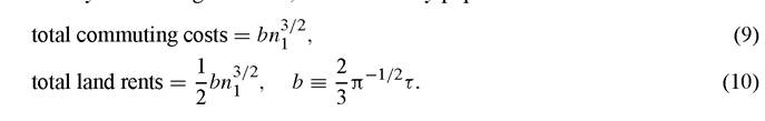
Equation (9) represents the key resource costs, where marginal commuting costs are increasing in city population. Rents are income to, potentially, a city developer or to rentiers.

How do cities form and how are sizes determined? We start with a specific mechanism and discuss how it generalizes below, and what happens if such a mechanism is not present. There is an unexhausted supply of identical city sites in the economy, each owned by a land developer in a nationally competitive urban land development market. A developer for an occupied city collects local land rents, specifies city population (but there is free migration in equilibrium), and offers any inducements to firms or people to locate in that city, in competition with other cities. Population is freely mobile.

The land developer maximizes

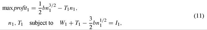
where T1 is the per firm subsidy (e.g., in practice, in a model with local public goods, a tax exemption), I1 is the real income per worker available in equilibrium in national labor markets under free mobility, which a single developer takes as given. In the con­straint, I1 equals wages in (7), plus the subsidy, less per worker rents plus commuting costs paid from (9) and (10). Maximizing with respect to T₁ and n₁ and imposing perfect competition in national land markets so profit₁ = 0 ex post, yields

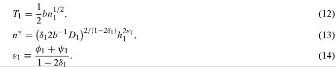
This solution has a variety of properties heralded in the urban literature. First it re­flects the Henry George Theorem [Flatters, Henderson and Mieszkowski (1974), Stiglitz (1977)], where the transfer per worker/firm exactly equals the gap (δ₁ W₁) between so­cial and private marginal of labor to the city, and that subsidy which prices externalities is exactly financed out of collected land rents at efficient city size.

By substituting in the constraint in (11), we can define relationships among real in­come, wages, and human capital. Substituting in first for T₁ and then n₁ we get

where Q₁ is a parameter cluster. Note real income is wages deflated by urban living costs; and that real income rises with human capital.

Institutions and city size. I have specified the equilibrium in national land markets, given competitive developers. Helsley and Strange (1990) put this in proper context, specifying the city development game, determining how many cities will form and what their sizes (n*) will be. Henderson and Becker (2001) show that the resulting solu­tions (with multiple factors of production) are (1) Pareto efficient, (2) the only coalition proof equilibria in the economy, (3) unique under appropriate parameters, and (4) free mobility ones where the developer specified populations are self-enforcing.

Absent such institutions, cities only form through “self-organization”. In the model here with perfect mobility of resources, the result is potentially enormously oversized cities [Henderson (1974), Henderson and Becker (2001)]. Nash equilibrium city size in atomistic worker migration decisions lies between efficient size, n*, and a limit size to the right, n_max, where city size is so large with such enormous diseconomies that the population is indifferent between being in a rural settlement of size 1 (the size of a community formed by a defecting migrant) and n_max. That is, given an inverted-U shape to real income I₁, self organization has cities at the right of the peak n*, potentially at n_max where I₁ (n = 1) = I₁ (n = n_max). The problem is the familiar one of co­ordination failure.

Consider a large economy with growing population, where, in size, all cities are at or just beyond n*. Timely formation of the next city to accommodate this population growth requires en mass movement of population from existing cities into a new city of size n*. Without co-ordination in the form of developers or city governments, no such en mass movement is possible, so people wait to migrate from existing cities to a new city until existing cities have all grown to n_max, where it pays individual migrants to exit cities to set up their own tiny “city”. At that “bifurcation point” [Krugman (1991a)], in equilibrium these milling migrants coalesce into 1 or more new cities of size greater than or equal to n*, at which point, again, all then existing cities start to grow again with national population growth until they too hit the bifurcation point n_max. This dismal process is what faces countries where local autonomy and national markets are poorly functioning, so that there are no market or institutional mechanisms to co-ordinate en mass movements of people. However the process we have outlined involving popula­tion swings across cities and potentially enormously over-populated cities may not be consistent with the data. In Section 3 we will outline a model with immobile capital, where self-organization can involve “commitment” given irreversibility of investment decisions. In that context outcomes, while still inefficient, are not so dismal.

2.1.2. Other city types

In Black and Henderson (1999a), X₁ city type 1 is an input into production of the single final good in the economy X₂ (from which, hence in a growth context human capital is also “produced”). In many models all outputs of specialized city types are final con­sumption goods. But here we follow Black and Henderson, without loss of generality. X₂ is produced in type 2 cities where the output for worker/firm j is correspondingly,

As in type 1 cities, per worker output is subject to own industry local scale externalities and to local knowledge spillovers. However now there is an intermediate input X₁ j, which is the numeraire good, with X₂j priced at P in national markets. The analysis of city sizes and formation for type 2 cities proceeds as for city type 1, with corresponding expressions, other than the addition of an expression for P in n₂ and I₂ and a restriction for an inverted-U shape to I₂ that δ₂ < α/2.

In a static context the model is closed by utilizing the national full employment con­straint

where m₁ and m₂ are the numbers of each type of city and N is national population. The second equation (to solve the 3 unknowns P, m₁ and m₂) equates real incomes as in Equation (15) across cities (I₁ = I₂), where individual workers move across cities to equalize real incomes. Finally, there is an equation where national demand equals sup­ply in either the market. That is, the supply, m₁ X₁, equals the demand for X₁ as an in­termediate input, m₂n₂x₁, and for producing commuting costs (m₁ (bn³1/²) + m₂ (bn³₂ ²)) from Equation (9). In this specific model, the solution yields values of m₁, m₂ and P that are functions of parameters and h₁ and h₂. In a static context of identical work­ers, one would impose h = h₁ = h₂. We will discuss momentarily the solution for h₁ and h₂ and the model in the growth context. Later in Section 3, we will detail solu­tions for prices and numbers of cities in a simpler but related two sector model. Here given log-linear production functions and a single final consumption good, as Black and Henderson show, X₁ /X₂ and m₁ /m₂ will be constant over time, independent of h.

In the static context where, labor mobility requires I1 = I2, in the larger type of city, say type 1, commuting and land rent costs will be higher. Thus, if real incomes

are equalized, from (15), Ψ₁ > W₂ as a compensating differential for higher living costs. Firms in type 1 cities are willing to pay higher wages because type 1 cities offer them greater scale benefits. Empirical evidence shows as cities move from a small size (say, 50,000) to very large metro areas, the cost-of-living typically doubles [Thomas (1978) and Henderson (2002)], explaining the fact that nominal wages also double.

Another issue discussed at length in Section 1.3 is that policy makers may favor large cities because they view them as “more productive”. Indeed for an industry found in smaller towns, it may be that the externalities they face in Equations (6) or (16) may be higher in a larger city. However that does not mean they locate there. Although externalities may be higher, in order for them to locate there, it must be sufficiently relatively higher to afford the higher wage and land rents, compared to a smaller city. If not, their profit maximizing or cost minimizing location is the smaller city.

Specialization. This analysis presumes cities specialize in production. That is an equi­librium outcome under a variety of conditions. In the model described so far, there are no costs of inter-city trade: no costs of shipping X₁ as inputs to X₂ type cities and ship­ping X₂ back as retail goods in X₁ type cities. All transport costs are internal to the city, given the relative greater importance of commuting costs in modern economies. Given that and given scale economies are internal to the industry, any specialized city (formed by a developer) out-competes any mixed city. The heuristic argument is simple. Con­sider any mixed city with n₁ and n₂ workers in industry 1 and 2. Split that city into two specialized cities, one with just n₁ people and the other with just n₂. Scale economies are undiminished (n∣^{i 1} and n^δ₁² in both cases in industries 1 and 2, respectively) but per worker commuting costs are lower in the specialized cities compared to the old larger mixed cities, so real incomes are higher in each specialized city compared to the old city.

Having own industry, or localization economies is a sufficient but not necessary condition for specialization. Industries can instead all have “urbanization” economies where scale depends on total local employment. However if the degree of urbanization economies differs across industries, then each industry has a different efficient local scale and is better off in a different size specialized city than any mixed city. Mixed cities occur more in situations where each good has localization economies enhanced by separate spillovers from the other industry or sharing of some common public in­frastructure [Abdel-Rahman (2000)].

A basic problem in these urban models is the lack of nuance on transport costs. Either transport costs of goods across cities is zero or infinite as for housing, and potentially other nontradables. A recent innovation is to have generalized transport costs (without a specific geography) where the cost of transporting a unit of X₁ to an X₂ city is t₁ and the cost of shipping X₂ back to an X₁ city is t₂, an innovation due to Abdel-Rahman (1996) in a model similar to the one used here (one intermediate and one final good) and then generalized by Xiong (1998) and Anas and Xiong (1999). Now whether there are specialized as opposed to diversified cities depends on the level of t₁ and t₂. At ap­propriate points as t₁ or t₂ or both rise from zero, X₁ and X₂ will collocate (in developer run cities) in one type of city, while there may be some cities specialized in one of either X₁ or X₂. More generally with a spectrum of, say, final products, we would expect that some products with low enough t's will always be produced in specialized cities, some high enough t's will be in all cities, and some with middle range t's will be produced in some cities (ones with bigger markets) but not others (with smaller markets). No one has yet simulated this more complex outcome.

2.1.1. Replicability and national policy

At the national level in a large economy with many cities, at the limit, there are con­stant returns to scale, or replicability. If national population doubles, the numbers of cities of each type and national output of each good simply doubles, with individ­ual city sizes, relative prices and real incomes unchanged.^[377] With two goods and two factors, basic international trade theorems (Rybczynski, factor price equalization, and Stolper-Samuelson) hold [Hochman (1977), Henderson (1988)]. This gives an urban flavor to national policies [Renaud (1981), Henderson (1988)]. For example trade pro­tection policies favoring industry X₁ produced in relatively large size cities over indus­try X₂ produced in smaller type cities will alter national output composition towards X1 production and increase the number of large relative to small cities. National urban concentration will rise. Similarly subsidizing an input such as capital for a high tech product, X₁, again, say, produced in a larger type of city will cause the numbers of that type of city to increase, raising urban concentration.

2.2. Growth in a system of cities

Black and Henderson (1999a) specify a dynastic growth model where dynastic families grow in numbers at rate g over time starting from size 1. If c is per person family consumption, the objective function is /0“ ^è'1__σ^-1 e^-(^ρ-g) dt where p (> g) is the discount rate. Dynasties can splinter (as long as they share their capital stock on an equal per capita basis) and the problem can be put in an overlapping generations context with equivalent results [Black (2000)], under a Galor and Zeira (1993) “joy of giving” bequest motive.

The only capital in the model is human capital and as such there is no market for it. Intra-family behavior substitutes for a capital market. Specifically families allocate their total stock of human capital (H) and members across cities, where Z proportion of family members go to type 1 cities (taking Zh₁e^gt of the H with them) and (1 - Z) go to type 2 cities [taking (1 - Z')h₂e^gt with them]. Additions to the family stock come from the equation of motion where the cost of additions, PHl, equals family income Ze^gt I₁ + (1- Z)e^gt I₂, less the value of family consumption of X₂, or Pce^gt. Constraints prohibiting consumption of human capital, nontransferability except to newborns, and nontransferability within families across city types (either directly or indirectly through migration) are nonbinding on equilibrium paths.

Families allocate their populations across types of cities, with low human capital types (say h₁) “lending” some of their share (h = H∕e^gt) to high human capital types (say h₂). High human capital types with higher incomes (I₂ > I₁ if h₂ > h ₁) repay low human capital types so c₁ = c₂ = c (governed by the family matriarch). This in itself is an interesting development story, where rural families diversify migration destinations (including the own rural village) and remittances home are a substantial part of earnings. In Black and Henderson if capital markets operate perfectly for human capital (i.e., we violate the “no slavery” constraint) or capital is physical and capital markets operational, one dynastic family could move entirely to, say, type 1 cities and lend some of their human capital to another dynastic family in type 2 cities. With no capital market, each dynastic family must operate as its own informal capital market and spread itself across cities.

In this context Black and Henderson show that, regardless of scale or timing in the growth process, h₁∕h₂ and I₁ /I₂ are fixed ratios, dependent on θ_i in Equations (6) and (16). As θ₁ ∕θ₂ (the relative returns to capital) rises, h₁∕h₂, I₁ /I₂ and also n₁ ∕n₂ rise. Z and m₁∕m₂ are all fixed ratios of parameters θ_i, δ_i and α under equilibrium growth. Equilibrium and optimal growth differ because the private returns to educa­tion in a city, θ_i, differ from the social returns, θ_i + ψ_i. But local governments cannot intervene successfully to encourage optimal growth. Why? With free migration and “no slavery”, if a city invests to increase its citizens’ education, a person can take their human capital (“brain drain”) and move to another city (be subsidized by another city to immigrate, given that city then need not provide extra education for that worker). This model hazard problem discourages internalization of education externalities.

2.2.1. Growth properties: cities

From Equation (13), equilibrium (and efficient) city size in type 1 cities is a function of the per person human capital level, h₁, in type 1 cities. After solving out the model (for P), the same will be true of type 2 cities. City sizes grow as h₁ and h₂ grow, where, under equilibrium growth given h₁∕h₂ is a fixed ratio, h ₁∕h₁ = h₂∕h₂ where a dot represents a time derivative. Then

where n_i ∕n_i is the growth rate of efficient sizes n*.

For the number of cities, the issue is whether growth in individual sizes absorbs the national population growth, or more cities are needed. Given

the numbers of cities grow if g > n_i∕n_i. Note growth in numbers and sizes of cities is “parallel” by type, so the relative size distribution of cities is constant overtime. Parallel growth with a constant relative size distribution of cities as reviewed in Section 1.1 is what is observed in the data. This result generalizes to many types of cities under certain conditions. For example, with the log-linear production technologies we assumed and with many varieties of output consumed under unitary price and income elasticities of log-linear preferences, parallel growth results.

2.2.1. Growth properties: economy

Ruling out explosive or divergent growth, there are two types of growth equilibria. Either the economy converges to a steady-state level, or it experiences endogenous steady-state growth. Convergence to a level occurs if ε ? ε₁(1 - (α — 2δ2)) + ε₂(α — 2δ₂) < 1, where ε is a weighted average of the individual city type. In that case at the steady-state h, n_i∕n_i = 0 and mi_i∕m_i = g, or only the num­bers but not sizes of cities grow just like in exogenous growth [Kanemoto (1980), Henderson and Ioannides (1981)]. If ε = 1 then there is steady-state growth, where γ^h = hi/h = (A — ρ)∕σ (where the transversality condition requires A > p). In that case n_i∕n_i = 2ε₁(A — ρ)∕σ, or cities grow at a constant rate. and their numbers also increase if g > 2ε₁(A — ρ)∕σ. This “knife-edge” formulation of whether there is en­dogenous growth or not dependent on the value of ε is not essential. For example in Rossi-Hansberg and Wright (2004) endogenous growth can occur more generally in a context where human capital accumulation involves worker time and the growth rate of human capital is a log-linear function of the fraction of time devoted to human capital accumulation, as opposed to production.

2.3. Extensions

There are three major extensions to the basic systems of cities models. First people may differ in terms of inherent productivity or in terms of endowments. Second, while we have discussed the issue of city specialization versus diversification, we have not developed insights into a more nuanced role of small highly specialized cities versus large diversified metro areas in an economy.

2.3.1. Different types of workers

Turning to the first extension, Henderson (1974) has physical capital as a factor of pro­duction owned by capitalists who need not reside in cities. Equilibrium city size reflects a market trade-off between the interests of city workers who have an inverted-U shape to utility as a function of the size of the city they live in and capitalists whose returns to capital rise indefinitely with city size (for the same capital to labor ratio). There is a political economy story, where capitalists collectively in an economy have an incen­tive to limit the number of cities, thus forcing larger city sizes. Helsley and Strange (1990) have a matching model between the attributes of entrepreneurs and workers and Henderson and Becker (2001) a related two class model. Again the two class model yields a conflict between the city sizes that maximize the welfare of one versus another group, which is resolved in competitive national land development markets.

In a different approach Abdel-Rahman and Wang (1997), Abdel-Rahman (2000) and later Black (2000) look at high and low skill workers who are used in differing propor­tions in production of different goods. Black has one traded good produced with just low skill labor and a second traded good produced with high skill workers and inputs of a local nontraded good produced with just low skill workers. High skill workers gen­erate production externalities in the form of knowledge spillovers for all traded goods. In Black, urban specialization with all high skill workers (and some low skill work­ers) concentrated in one type of city producing the first type of good is efficient; but a separating equilibrium that would sustain this pattern, where low skill workers and low tech production stay in their own type of city (rather than trying to cluster with high tech production) is not always sustainable. Black characterizes conditions under which a separating equilibrium will emerge.

It is important to note that there is a much more developed literature on inequality induced by neighborhood selection, where the characteristics of neighbors affect skill acquisition (e.g. average family background in the classroom affects individual student performance). That leads to segregation of talented or wealthier families by neighbor­hood [Benabou (1993), Durlauf (1996)] and can help transmit economic status across generations, promoting inter-generational income inequality.

2.3.2. Metro areas

Simple indices of urban diversity indicate that smaller cities are very specialized and larger cities highly diversified. So the question is what is the role of large metro areas in an economy and their relationship to smaller cities. Henderson (1988) and Duranton (2005) have a first nature - second nature world, where every city has a first nature economic base and footloose industries cluster in these different first nature cities. In general the largest centers are those attracting the most footloose production to their first nature center. The Duranton paper is discussed in more detail in Section 2.3.3. However, it seems that today few metro areas have an economic base of first nature activity. Accordingly recent literature has focused on the role of large metro areas as centers of innovation, headquarters, and business services [Kolko (1999)].

The Dixit-Stiglitz model opened up an avenue to look at large metro areas as having a base of diversified intermediate service inputs, which generate scale-diversity bene­fits for local final goods producers. That initial idea was developed in Abdel-Rahman and Fujita (1990) and has led to a set of papers focused on the general issue of what activities, under what circumstances are out-sourced. Theory and empirical evidence [Holmes (1999) and Ono (2000)] suggest that as local market scale increases, final pro­ducers will in-house less of their service functions. The resulting increased out-sourcing encourages competition and diversity in the local business service market, encouraging further out-sourcing.

In terms of incorporating this into the role of metro areas versus smaller cities, Davis (2000) has a two-region model, a coastal internationally exporting region and an interior natural resource rich region. There are specialized manufacturing activities which, for production and final sale, require business service activities, summarized as headquar­ters functions. Headquarters purchase local Dixit-Stiglitz intermediate services such as R&D, marketing, financing, exporting, and so on. Headquarters’ activity is in port cities in the coastal region. The issue is whether manufacturing activities are also in these ports versus in specialized coastal hinterland cities versus in specialized interior cities. If the costs of interaction (shipping manufactured goods to port and transac­tions costs of headquarters-production facility communication) between headquarters and manufacturing functions are extremely high, then both manufacturing and head­quarters activities will be found together in coastal port cities. Otherwise they will be in separate types of cities where manufacturing cities will be in coastal hinterlands if costs of headquarters-manufacturing interaction are high, relative to shipping natural resources to the coast. However if natural resource shipping costs are relatively high, then manufacturing cities will be found in the interior. Duranton and Puga (2001) have a very similar model of functional specialization, without the regional flavor. If there is specialization, then there are headquarter cities where headquarters outsource local services in diversified large metro areas, while production occurs in specialized manu­facturing cities.

In a different paper Duranton and Puga (2000) develop an entirely different and stim­ulating view of large metro areas. In an economy there are m types of workers who have skills each specific to producing one of m products. Specialized cities have one type of worker producing the standardized product for that type of worker subject to localization economies. Diversified cities have some of all types of workers. Existing firms at any instant die at an exogenously given rate; and, in a steady-state, new firms are their replacement. New firms do not know “their type” - what types of workers they match best with and hence what final product they would be best off producing. To find their type they need to experiment by trying the different technologies (and hence trying different kinds of workers). New firms have a choice. They can locate in a diver­sified city with low localization economies in any one sector. But in a diversified city they can experiment with a new process each period until they find their ideal process. At that point they relocate to a city specialized in that product, with thus high local­ization economies for that product. Alternatively new firms can experiment by moving from specialized city to specialized city with high localization economies, but face a re­location cost each time. If relocation costs are high, it is best during their experimental period to be in a diversified city. This leads to an urban configuration of experimental diversified metro areas and other cities which are specialized in different standardized manufacturing products.

The Duranton and Puga model captures a key role of large diversified metro areas consistent with the data. They are incubators where new products are born and where new firms learn. Once firms have matured then they typically do relocate to more spe­cialized cities. This also captures the product-life cycle for firms in terms of location patterns. Fujita and Ishii (1994) document the location patterns of Japanese and Korean electronics plants and headquarters. In a spatial hierarchy megacities house headquarters activities (out-sourcing business services) and experimental activity. Smaller Japanese or Korean towns have specialized, more standardized high tech production processes and low tech activity is off-shore.

2.3.3. Stochastic process and Zipf's Law

Gabaix (1999a, 1999b) argues that if, there is a stochastic process where individual city growth rates follow Gibrat’s Law - the growth rate in any period is unrelated to initial size - then the size distribution that emerges will follow Zipf’s Law. Beyond specifying a stochastic process where shocks to productivity or preferences follow a random walk, to get the result in a model where there is an endogenous number of cities of efficient sizes, as opposed to just fixing the number of cities [Gabaix (1999a) and Duranton (2005)] requires considerable structure, with a variety of such issues be­ing analyzed in Cordoba (2004). We follow Rossi-Hansberg and Wright (2004) who adapt the model we have presented. In their base case there is only human capital; and technology and preferences are log-linear. They have many final output industries and hence types of specialized cities. They group industries and specialized city types into sets. Within each set industries and city types have the same technology but each in­dividual industry draws its own permanent shock each instant. In terms of the shock they assume that D₁ (t) in the equivalent of Equation (6) follows a finite-order Markov process. Finally and critically to have Gibrat’s Law lead to Zipf’s Law, they must im­pose an arbitrary lower bound on the sizes that cities can fall to [Gabaix (1999a)]. These assumptions lead to Zipf’s Law holding for each set of industries and they show one can aggregate across sets of industries to get Zipf’s Law in aggregate. It goes without saying many of the assumptions imposed to get Zipf’s Law are very strong, a key point made in Cordoba (2004).

In a recent paper, Duranton (2005) tries to model “micro-foundations” for the sto­chastic process affecting city sizes and as a result ends up modeling an important overlooked aspect of city evolution. Duranton has “first nature” (immobile given natural resource location) production and “second nature” (mobile, or footloose) production in m cities, where m is given by the number of immobile natural resource products, each needing their own city. So, in contrast to Rossi-Hansberg and Wright the number of cities is fixed; but given that restriction a lot is accomplished. In the paper there are (n » m) products, in a Grossman and Helpman (1991) product quality ladder model. The latest innovation in each product is produced by the monopolist holding the patent and only this top quality is marketed for any product. Investment in innovation to try to move the next step up in the quality ladder in industry k and get the next patent in k, can also lead to the next step up in a different industry - i.e., there can be cross-industry innovation. For footloose industries, to partake of a winning innovation occurring for industry k in city i, requires industry k production to locate in city i where the inno­vator is. Presumably co-location of the inventor and production makes the information needed for the transition to mass production cheaper to exchange (e.g., the workers in the innovative firm take over production). Innovation follows a stochastic process where innovation probabilities depend on R&D expenditures. Industry jumps from city to city according to where the latest innovation is, and city growth also follow a stochastic process. The resulting stochastic process of city growth and decline results in steady state size distributions that are similar to Zipf’s Law. Adding in considerations of urban scale economies in the innovation process helps explain the long right tails in actual city size distributions, as they differ from Zipf’s Law.

Duranton’s formulation has the nice feature that cities have patterns of production specialization which change over time. This seems to fit the data; and Duranton’s pa­per in fact models the evolution of industry structure of cities. We know from Black and Henderson (1999b) and Ellison and Glaeser (1999b) that industries move “rapidly” across cities, with city specialization changing over time for cities. Any city is very slow to gain a high share of any particular industry’s production (given there are many possible industries to gain a share from) and is very quick to lose a high share (given many competitor cities).

3.