Facts and empirical evidence
This section reviews basic facts and a body of empirical evidence on systems of cities. We start by looking at evidence based primarily on either the world as a whole or on large developed countries.
We look at the evolution of the size distribution of cities, Zipf’s Law and related topics. Then we turn to what cities do - evidence on urban specialization and geographic concentration - and where they locate. Finally we turn to evidence that is more specific to the urbanization process in developing countries and issues surrounding that process.1.1. The size distribution of cities and its evolution
Work by Eaton and Eckstein (1997) on France and Japan and by Dobkins and Ioannides (2001) on the USA, with later work by Black and Henderson (2003) and Ioannides and Overman (2003) on the USA, establish some basic facts about urban systems and their development in France, Japan and the USA over the last century or so. Foremost is that there is a wide relative size distribution of cities in large economies that is stable over time. Big and small cities coexist in equal proportions over long periods of time. Second, within that relative size distribution, individual cities are generally growing in population size over time; and what is considered a big versus small city in absolute size changes over time. Third, while there is entry of new cities and both rapid growth and decline of cities nearer the bottom of the urban hierarchy, at the top city size rankings are remarkably stable over time. Finally, size distributions of cities within countries, at least at the upper tail are well approximated by a Pareto distribution, with Zipf’s Law applying in many cases. Establishing these facts raises a variety of issues and different methodological and technical approaches.
1.1.1. What is a city?
The empirical work in Eaton and Eckstein (1997) and subsequent work typically looks at the decade by decade development of urban systems.
In doing so, there are critical choices researchers must make when assembling data. First is to define geographically what consists of the generic term “city”. The usual definition is the “metro area”, where large metro areas like Chicago comprise over 100 municipalities, or local political units. The idea in defining metro areas is to cover the entire local labor market and all contiguous manufacturing, service and residential activities radiating out from the core city, until activity peters out into farm land or very low density development. A second choice concerns how to accommodate changes in geographic definitions over time. One can use whatever contemporaneous definitions the country census/statistical bureau uses; however metro area definitions only start to be applied after World War II. Another approach is to take current metro area definitions and follow the same geographic areas back in time, focusing on nonagricultural activity.A third problem concerns how to define “consistently” over time the threshold population size at which an agglomeration becomes a metro area, especially since the economic nature, population density, and spatial development of metro areas have changed so much over the last century. Some authors use an absolute cut-off point (e.g., urban population of 50,000 or more); some use a relative cut-off point (e.g., the minimum size city included in the sample should be 0.15 mean city size); and others look at a set number (e.g., 50 or 100) of the largest cities. The relative cut-off point approach is attractive because it attempts to hold constant the area of the relative size distribution which is examined over time, as illustrated below. In presenting evidence on the topics to follow, whatever choices researchers make can strongly affect specific results. Nevertheless there are a variety of findings that are consistent across studies.
1.1.2. Evolution of the size distribution
In the research, one focus has been to study the evolution of the size distribution of cities, applying techniques utilized by Quah (1993) in examining cross-country growth patterns.
Cities in each decade are divided by relative size into, say, 5-6 discrete categories, with fixed relative size cut-off points for each cell (e.g., 2.2 mean size). A first-order Markov process is assumed and a transition matrix calculated. In many cases, stationarity of the matrix over decades cannot be rejected, so cell transition probabilities are based on all transitions over time. If M is the transition matrix, i the average rate of entry of new cities in each decade (in a context where in practice there is no exit), Z the (stationary) distribution across cells of entrants (typically concentrated on the lowest cell), and f the steady-state distribution, then
Inthe data, relative size distributions are remarkably stable overtime and steady-state distributions tend to be close to the most recent distributions. In the studies on the USA, Japan and France, there is no tendency of distributions to collapse and concentrate in one cell, or for all cities to converge to mean size; nor generally is there a tendency for distributions to become bipolar. Distributions are remarkably stable. I illustrate this based on a world cities analysis (although, conceptually, distributions may better apply to countries, within which populations are relatively mobile).
Table 1 gives the size distribution of world metro areas over 100,000 population in 2000. Details on the data are available on-line.1 Note that much of the world’s pop-
Table 1
World city size distribution, 2000
| Size range | Count | Mean | Share* |
| 17,000,000 ≤ n2000 | 4 | 20,099,000 | 4.5 |
| 12,000,000 ≤ n2000 < 17,000,000 | 7 | 13,412,714 | 5.2 |
| 8,000,000 ≤ n2000 < 12,000,000 | 13 | 10,446,385 | 7.5 |
| 4,000,000 ≤ n2000 < 8,000,000 | 29 | 5,514,207 | 8.9 |
| 3,000,000 ≤ n2000 < 4,000,000 | 41 | 3,442,461 | 7.8 |
| 2,000,000 ≤ n2000 < 3,000,000 | 75 | 2,429,450 | 10.1 |
| 1,000,000 ≤ n2000 < 2,000,000 | 247 | 1,372,582 | 18.8 |
| 500,000 ≤ n2000 < 1,000,000 | 355 | 703,095 | 13.9 |
| 250,000 ≤ n2000 < 500,000 | 646 | 349,745 | 12.5 |
| 100,000 ≤ n2000 < 250,000 | 1,240 | 157,205 | 10.8 |
| Overall | 2,657 | 658,218 | 100.0 |
* A ratio of total population in the group to total population of cities with ≥ 100,000.
1
http://www. econ.brown.edu/faculty/henderson/worldcities.html.
ulation in cities over 100,000 are in small-medium size metro areas. 56% are in cities under 2 million, while only 17% are in cities over 8 million. Moreover, all these cities only account for 62% of the world’s urban population; the rest live in cities smaller than 100,000. So overall 73% of the world’s urban population lives in cities under 2 million in population. While the popular press may focus on megacities, only a small part of the action is there.
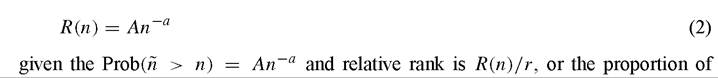
Figure 1 plots the relative size distribution of the approximately 1200 metro areas worldwide over 100,000 in 1960 against the relative size distribution of the approximately 1700 metro areas over 200,000 in 2000. Relative sizes are actual sizes divided by the world average size in the corresponding year. The 100,000 versus 200,000 cut-off points for minimum size are relative ones based on a constant minimum to mean size ratio. (Although using an absolute cut-off point in this case has little impact on the figure.) The figure plots the histogram for 20 cells on a log scale. The 1960 versus 2000 distributions for all cities worldwide [Figure 1(a)] and for those in developing and transition economies [Figure 1(b)] almost perfectly overlap. Relative size distributions are stable. Similarly performing transition analysis on world cities for 1960-1970-1980-19902000 and calculating the steady state distributions, starting with 5 cells and shares in each of 0.351, 0.299, 0.151, 0.100, 0.0991 in 1960, as we move up the urban hierarchy the steady state shares are 0.324, 0.299, 0.138, 0.122 and 0.117. Again, this indicates rock stability of distributions over time.
Analternative way of expressing this is to calculate spatial Gini’s [Krugman (1991b)]. For a spatial Gini rank all cities from smallest to largest on the x-axis and on the y-axis calculate their Lorenz curve - the cumulative share of total sample population. The Gini is the share of the area below the 45o line, between that line and the Lorenz curve.
The greater the Gini, the “less equal” the size distribution. The world Gini in 1960 versus 2000 is 0.59 versus 0.56 for developed countries, 0.57 versus 0.56 for less developed countries, and 0.52 versus 0.45 for transition economies as noted in Table 2 columns (1)-(4). Table 2 also lists Gini’s for 1960 versus 2000 for 14 countries. Note apart from transition economies (and Nigeria), the lack of change; and note also that transition economies are distinctly “more equal”. Transition economies have forestalled the growth of megacities through explicit and implicit (housing availability in cities) migration restrictions, as discussed in Section 3.3.1.A second finding in examining city size distributions is that, for larger cities, over time there is little change in relative size rankings. In Japan and France, the 39-40 largest cities in 1925 and 1876, respectively, all remain in the top 50 in 1985 and 1990 respectively; and, at the top, absolute rankings are unchanged [Eaton and Eckstein (1997)]. The USA displays more mobility due to substantial entry of new cities. However, while smaller cities do move up and down in rank, the biggest cities tend to remain big over time. So, for example, cities in the top decile of ranking stay in that decile indefinitely, with newer cities joining that decile as the total number of cities expands. Alternatively viewed, based on the Markov transition process, the mean first passage time for a city to move from the top to bottom cell is thousands of years [Black and Henderson (2003)]. In the world cities data, as in the USA data, the probability in the transition matrix of mov-
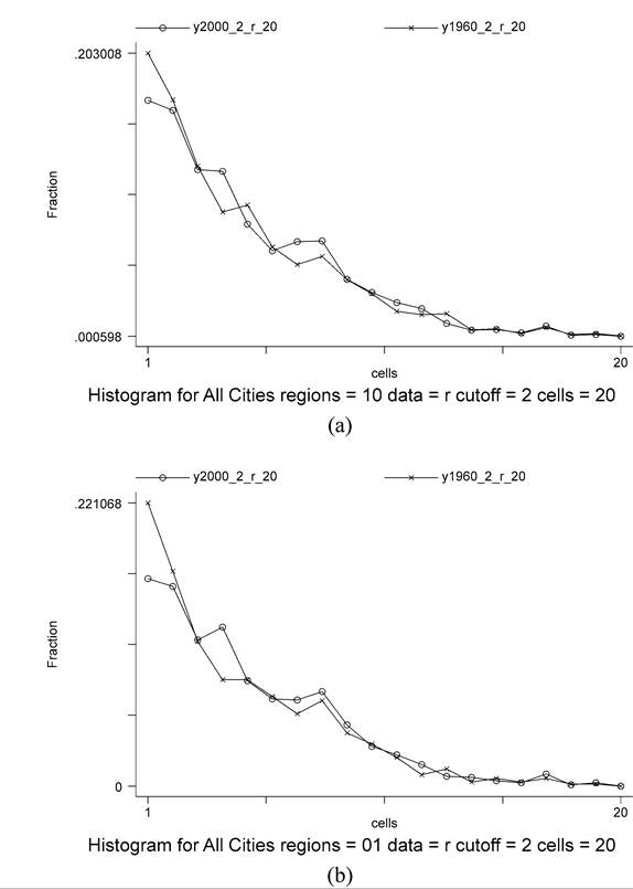
Figure 1. (a) Relative size distribution of cities for all countries. (b) Relative size distribution of cities in developing and transition economies.
ing out of the top cell to the next cell is very small: 0.038 in a decade time frame. Why do big cities stay big? A common answer is physical infrastructure (see Section 3.3.2).
Large cities have huge historical capital stocks of streets, buildings, sewers, water mains and parks that are cheaply maintained and almost infinitely lived, that give them a persistent comparative advantage over cities without that built-up stock. A second answer is modeled in Arthur (1990) and Rauch (1993) where, with localized scale externalities inTable 2
Spatial inequality
| 1960 | 2000 | ||||
| Gini (1) | Number of cities (2) | Gini (3) | bgcolor=white>Number of cities Rank size coefficient “fl” (5) | ||
| World | 0.59 | 1197 | 0.56 | 1673 | n.a. |
| Developed | 0.65 | 523 | 0.58 | 480 | n.a. |
| Soviet bloc | 0.52 | 179 | 0.45 | 202 | n.a. |
| Less developed | 0.57 | 495 | 0.56 | 991 | n.a. |
| Brazil | 0.67 | 24 | 0.65 | 65 | -0.87 |
| China | 0.47 | 108 | 0.43 | 223 | -1.3 |
| India | 0.56 | 95 | 0.58 | 138 | -1.1 |
| Indonesia | 0.52 | 22 | 0.61 | 30 | -0.90 |
| Mexico | 0.61 | 28 | 0.60 | 55 | -1.04 |
| Nigeria | 0.31 | 20 | 0.60 | 38 | -0.98 |
| France | 0.61 | 31 | 0.59 | 27 | -0.97 |
| Germany | 0.60 | 44 | 0.56 | 31 | -0.74 |
| Japan | 0.60 | 100 | 0.66 | 82 | -1.06 |
| Russia | 0.54 | 79 | 0.46 | 91 | -1.34 |
| Spain | 0.53 | 27 | 0.52 | 20 | -0.98 |
| Ukraine | 0.44 | 25 | 0.40 | 32 | -1.31 |
| UK | 0.68 | 39 | 0.60 | 21 | -0.83 |
| USA | 0.58 | 167 | 0.54 | 197 | -1.11 |
production, large cities with a particular set of industries have a comparative advantage in attracting new firms, relative to cities with a small representation of those industries. Large cities have an established scale, offering high levels of scale externalities, which smaller cities can only achieve quickly if they are able to co-ordinate mass in-migration of firms into their location, something which may be institutionally difficult to do.
1.1.2. Growth in city numbers and sizes
For any steady state size distribution of cities, as urbanization and growth proceed, both the absolute sizes and numbers of cities have grown historically, as a country’s urban population expands through rural-urban migration and overall population growth. City sizes in the USA, Japan and France over the past century have grown at average annual rates of 1.2-1.5%, depending on the country and exact time interval, rates which involve city sizes rising 3.3-4.5 fold every century. A small city today which is 250,000 would have been a major center in 1900.
In the world city data set, for comparable sets of countries the numbers of metro areas grew by 62% from 1960-2000 using a relative cut-off point (approximately 100,000 in 1960 versus 170,000 for this sample in2000). Average sizes grew by about 70%. Decade by decade figures are given in Table 3. Using an absolute cut-off point of 100,000, num-
Table 3
Total numbers of cities and sizes
| 1960 | 1970 | 1980 | 1990 | 2000 | |
| Number of cities | 969 | 1,129 | 1,353 | 1,547 | 1,568 |
| Mean size | 556,503 | 640,874 | 699,642 | 789,348 | 943,693 |
| Median size | 252,539 | 275,749 | 304,414 | 355,660 | 423,282 |
| Minimum size | 100,082 | 115,181 | 126,074 | 141,896 | 169,682 |
bers have about doubled and average sizes grown by 36% over 40 years. However we count cities, it is clear they have grown in population and numbers on an on-going basis over the decades.
The theory section will model city size growth and numbers in developed, or fully urbanized countries in Section 2 and in urbanizing economies in Section 3, as related to technological change induced by knowledge accumulation and demographic changes. There is empirical work relating city size increases to changes in knowledge levels. Glaeser, Scheinkman and Schelifer (1995) in a cross-section city growth framework estimate that controlling for 1960 population, in the USA, cities in 1990 are 7% larger if they had a one-standard deviation higher level of median years of schooling in 1960. Black and Henderson (1999a) place the issue in a panel context for 1940-1990 for the USA controlling for city fixed effects and industrial composition; and they examine the impact of percent college educated (which has enormous time variation). They find a one-standard deviation increase in the percent college educated leads to a 20% increase in city size over a decade.
1.1.4. ZipfS Law
In considering the size distribution of cities, especially in a cross-sectional context, there is a large literature on what is termed Zipf’s Law [e.g., Rosen and Resnick (1980), Clark and Stabler (1991), Mills and Hamilton (1994) and Ioannides and Overman (2003)]. City sizes are postulated to follow a Pareto distribution, where if R is rank from smallest r, to largest 1, and n is size
cities with size greater than n. Under Zipf’s Law a = 1, or we have the rank size rule where, for every city, rank times size is a constant, A. Putting (2) in log-linear form, empirical work produces a ’s that vary across countries, samples and times; but many are “close” to one. This empirical regularity has drawn considerable attention and is often used to characterize spatial inequality, using (2) as a first approximation of the true size distribution. We list sample a coefficients for 2000 for fifteen countries in Table 2, column (5). Note however while people often say that an exponent of 0.74 or 1.34 is “close to” one, such coefficients produce very different city size distributions, than if the coefficient is one.[375] As a declines, or the slope of the rank size line gets flatter, urban concentration is viewed as increasing: for given size changes, rank changes more slowly, or cities are “less equal”. In Table 2, the a coefficients and the Gini’s are in fact strongly negatively correlated, as one would expect. But we note that typically the log version of Equation (2) is better approximated by a quadratic form than linear one. However one looks at it, Zipf’s Law is just an approximation that does well in some circumstances and not so well in others. If one wants to compare measures of urban concentration across countries or over time, rather than compare estimated a’s in Equation (2), using Gini’s may be more reliable, just as they are for comparisons of income distributions.
If Zipf’s Law holds even approximately, why is that? In an interesting development, Gabaix (1999a, 1999b) starts to formalize the underlying stochastic components which might lead to such a relationship, building on Simon (1955). Gabaix shows that if city growth rates obey Gibrat’s Law where growth rates are random draws from the same distribution,[376] so growth rates are independent of current size, Zipf’s Law emerges as the limiting size distribution (as long as a lower bound on how far cities can deteriorate in size is imposed). Growth is scale invariant, so the final distribution is; and we have a power law with exponent 1. Gabaix sketches an illustrative model, based on on-going natural amenity shocks facing cities of any size, which leads to Zipf’s Law for the size distribution of cities. More comprehensive formulations in Duranton (2005) and Rossi- Hansberg and Wright (2004) are discussed in the theory section.
ety of circumstance and subsamples, under appropriate statistical criteria, which rejects Gibrat’s Law. Ioannides and Overman (2003) examine the issue more thoroughly in a nonparametric fashion, characterizing the mean and variance of the distribution from which growth rates are drawn. The mean and variance of growth rates do seem to vary with city size but bootstrapped confidence intervals are fairly wide generally, allowing for the possibility of (almost) equal means.
1.2. Geographic concentration and urban specialization
 I
I

The distribution of qik across industries k, compared over time for a city would tell us about how city i’s specialization patterns are changing over time. And the distribution of qik across locations i, over time would tell us whether industry k is becoming more or less concentrated over time at different locations. In a practical applications looking at many industries and cities over time or across countries, the issue concerns how to produce summary measures to describe either how overall concentration varies across industries or how one city’s specialization compares with another’s. Another issue concerns how to factor in the different forces that cause specialization or concentration phenomena. The literature uses a variety of approaches. We start by looking at urban specialization.
1.2.1. Urbanspecialization
Evidence on countries such as Brazil, USA, Korea, and India [Helpman (1998) and Lee (1997)] indicate that cities are relatively specialized. The traditional urban specialization literature going back to Bergsman, Greenston and Healy (1972) uses cluster analysis to group cities into categories based on similarity of production patterns - correlations (or minimum distances) in the shares of different industries in local employment sik. Cluster analysis is an “art form” in the sense that there is no optimal set of clusters, and it is up to the researcher to define how fine or how broad the clusters should be and there are a variety of clustering algorithms.
Using 1990 data for the USA, Black and Henderson (2003) group 317 metro areas into 55 clusters, “defining” 55 city types based on patterns of specialization for 80 2-digit industries. They define textile, primary metals, machinery, electronics, oil and gas, transport equipment, health services, insurance, entertainment, diversified market center, and so on type cities, where anywhere from 5-33% of local employment is typically found in just one industry. They show that production patterns across the types are statistically different and that average cities and educational levels by type differ significantly across many of the types. Specialization especially among smaller cities tends to be absolute. At a 3-digit level many cities have absolutely zero employment in a variety of categories. So in the 1992 Census of Manufactures for major industries like computers, electronic components, aircraft, instruments, metal working machinery, special machinery, construction machinery, and refrigeration machinery and equipment, respectively, of 317 metro areas 40%, 17%, 42%, 15%, 77%, 15%, 14% and 24% have absolutely zero employment in these industries.
Kim (1995) in looking at the USA examines how patterns of specialization have changed over time, by comparing for pairs (i, j) of locations ∑k ∖sik - Sjk| and by estimating spatial Gini’s for industry concentration. He finds that states are substantially less specialized in 1987 than in 1860, but that localization, or concentration has increased over time. For Korea, as part of the deconcentration process noted earlier, Henderson, Lee and Lee (2001) find that from 1983 to 1993, city specialization as measured by a normalized Hirschman-Herfindahl index,

rises in manufacturing, while a provincial level index declines. Cities become more specialized and provinces less so. Clearly the geographic unit of analysis matters, as do the concepts. City specialization as envisioned in the models presented below is consistent with regional diversity, when large regions are composed of many cities of different types.
Henderson (1997) for the USA and Lee (1997) for Korea show that the gj index of specialization in manufacturing declines with metro area size. Smaller cities are much more specialized than larger cities in their manufacturing production. More generally, Kolko (1999) demonstrates that larger cities are more service oriented and smaller ones more manufacturing oriented. For six size categories (over 2.5 million, 1-2.5 million,... (2005), look at geographic concentration using British data. Rather than model the underlying stochastic process of industrial location under specific assumptions to yield a specific index, Duranton and Overman take a nonparametric approach, where they also focus on how to test statistically whether industries are significantly concentrated. They calculate the distribution of all pair-wise distances between plants in an industry. Distributions shifted to the left have a greater concentration of short pair-wise distances and are more spatially concentrated. The authors have the advantage of knowing “exact” plant locations (basically within a city block or so), rather than having to rely on, say, county locations, which in the US can cover vast distances. They develop a framework to test observed industry distributions against the “counterfactual” of what distributions would look like if firms choose locations randomly, given (a) the set of locations in the UK for industrial plants is limited, (b) bilateral distances between all possible points are not independent, and (c) industry sizes or numbers of plants differ. The framework involves repeated sampling for an industry without replacement from the set of national industrial sites with the sample size equal to industry size. Following that procedure, they construct 95% confidence intervals to test if observed distributions depart from randomness.
Compared to Ellison-Glaeser, in practical applications their approach captures a nu- anced aspect of spatial clustering. For relatively concentrated industries, the Ellison and Glaeser index is typically dominated by the county with the highest share (given squared shares in the index), telling us the extent to which an industry is concentrated in just one place. The Duranton-Overmanapproachtells us more generally about spatial clustering over the whole country. So in Ellison and Glaeser, an industry which has a high concentration in one county but is otherwise very dispersed across the 3000 USA counties may look more concentrated than an industry which is concentrated in, say 3-4 nearby
counties, with little representation elsewhere. But the latter would be well represented in Duranton and Overman.
1.2.3. Geography
A variety of recent studies have examined the role of geography, primarily natural features, in the spatial configuration of production and growth of cities. Rappaport and Sacks (2003) herald the role of coastline location in the USA, as a factor promoting city growth. In a related study, Beeson, DeJong and Troeskan (2001) look at USA counties from 1840-1990. They show that iron deposits, other mineral deposits, river location, ocean location, river confluence, heating degree days, cooling degree days, mountain location, and precipitation all affect the base 1840 county population significantly. However for 1840-1990 growth in county population, only ocean location, mountain location, precipitation, and river confluence matter, controlling for 1840 population. That is, first nature items strongly affected 1840 and hence indirectly 1990 populations; but growth from 1840-1990 is independent of many first nature influences. Ocean location as Sacks’ suggests has persistent growth effects.
Both these studies ignore the geography of markets and the role of neighbors in influencing city evolution. Dobkins and Ioannides (2001) show that growth of neighboring cities influences own city growth and cities with neighbors are generally larger than isolated cities. Black and Henderson (2003) put neighbor and geographic effects together. They calculate normalized market potential variables (sum of distance discounted populations of all other counties in each decade, normalized across decades). They find climate and coast affect relative city growth rates; but market potential has big effects as well, although they are nonlinear. Bigger markets provide more customers, but also more competition, so marginal market potential effects diminish as market potential increases. Highmarketpotential helps explain why North-East cities in the USA maintain reasonable growth, given for historical reasons, they are in the most densely populated area, despite the hypothesized natural advantages of the West.
1.3. Urbanization in developing countries
Urbanization, or the shift of population from rural to urban environments, is typically a transitory process, albeit one that is socially and culturally traumatic. As a country develops, it moves from labor-intensive agricultural production to labor being increasingly employed in industry and services. The latter are not land-intensive and are located in cities because of agglomeration economies. Thus urbanization moves populations from traditional rural environments with informal political and economic institutions to the relative anonymity and more formal institutions of urban settings. That in itself requires institutional development within a country. It spatially separates families, particularly by generation, as the young migrate to cities and the old stay behind.
Urbanization is a spatial transition process. By upper middle income ranges, countries become “fully” urbanized, in the sense that the percent urbanized levels out at
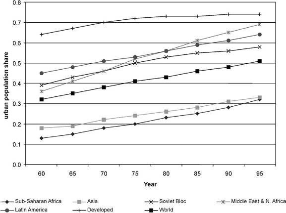
Figure 2. Share of urban population in total population. (Average over countries within groups.)
60-90% of the national population living in cities. The actual percent urbanized with full urbanization varies with geography, the role of modern agriculture in the economy, and national definitions of urban. This idea of a transitory phenomenon is illustrated Figure 2, comparing different regions of the world in 1960 versus 1995. While urbanization increased in all regions of the world over those 35 years, among developed countries there is little change since 1975. By 1995 Soviet bloc and Latin American countries had almost converged to developed country urbanization levels. Only Sub-Saharan African and Asian countries still face substantial urbanization in the future. Although urbanization is transitory, given the total spatial transformation and accompanying institutional and social transformation involved, as a policy issue, urbanization is very important to developing countries. Here we review some basic facts and issues about the process.
1.3.1. Issues concerning overall urbanization
As noted above, urbanization is the consequence of changes in national output composition from rural agriculture to urbanized modern manufacturing and service production. As such, Renaud (1981) makes the basic point that government policies bias, or influence urbanization through their effect on national sectoral composition. So policies affecting the terms of trade between agriculture and modern industry or between traditional small town industries (textiles, food processing) and high tech large city industries affect the rural-urban or small-big city allocation of population. Such policies include tariffs, and price controls and subsidies. The idea that government policies affect urbanization primarily through their effect on sector composition is a key point of empirical studies of Urbanizationby Fay and Opal (1999) and Davis and Henderson (2003). These studies show that, indeed, urbanization which occurs in the early and middle stages of development is determined largely by changes in national economic sector composition and in technology. Government policies tend to affect urbanization only indirectly through their effect on sector composition.
Urbanization promotes benefits from agglomeration such as localized information and knowledge spillovers and thus efficient urbanization promotes economic growth. Writers such as Gallup, Sachs and Mellinger (1999) go further to suggest that urbanization may “cause” economic growth, rather than just emerge as part of the growth process. The limited evidence so far suggests urbanization does not cause growth per se. Henderson (2003) finds no econometric evidence linking the extent of urbanization to either economic or productivity growth or levels. That is, if a country were to enact policies to encourage urbanization per se, typically that would not improve growth.
Finally on urbanization, there is an informal notion [Mills and Becker (1986) and World Bank (2000)] that the transitory urbanization process follows the same stages as population growth (the “demographic” transition between falling death rates and falling fertility rates) - an S-shaped relationship where urban population growth is slow at low levels of development, then there is a period of rapid acceleration in intermediate stages, followed by a slowing of growth. However the data suggest otherwise at least over the last 35 years. Figure 3 illustrates after parceling out the effect of national population, or country size, based on pooled country data every 5 years from 1965-1995. In Figure 3 the log of national urban population is an increasing concave function of the log of income per capita, indicating the growth rate of urban population is a concave increasing function of income levels [Davis and Henderson (2003)].
1.3.2. The form of urbanization: the degree of spatial concentration
In 1965, Williamson (1965) published an innovative paper based on cross-section analysis of 24 countries in which he argued that national economic development is characterized by an initial phase of internal regional divergence, followed by a phase of later convergence. That is, a few regions initially experience accelerated growth relative to other (peripheral) regions, but later the peripheral regions start to catch up. Barro and Sala-i-Martin (1991, 1992) present extensive evidence on this for the USA, Western Europe and Japan, by examining the evolution of inter-regional differences in per capita incomes. While inter-regional out-migration from poorer regions plays a role in catch-up, it may not be critical. For Japan, the authors argue that later convergence of backward regions occurred mostly through improved productivity in backward regions.
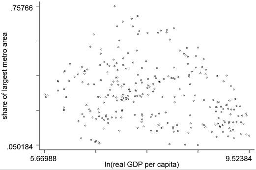
The urban version of this divergence-convergence phenomenon looks at urban primacy. Following Ades and Glaeser (1995), conceptually the urban world is collapsed into two regions - the primate city versus the rest of the country, or at least the urban portion thereof. The basic question concerns to what extent urbanization is concentrated, or confined to one (or a few) major metro areas, relative to being spread more evenly
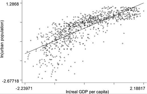
Figure 3. Partial correlation between ln(urban population) and ln(real GDP per capita), controlling for ln(national population), 1965-1995.
across a variety of cities. Primacy is commonly measured by the ratio of the population of the largest metro area to all urban population in the country [Ades and Glaeser (1995), Junius (1999) and Davis and Henderson (2003)]. A more comprehensive measure might use either a spatial Gini or a Hirschman-Herfindahl index (HHI) from the industrial organization literature.
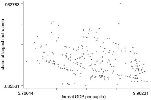
Corresponding to Williamson's hypothesis, these papers find an inverted-U-shape relationship, where relative urban concentration first increases, peaks, and then declines with economic development. Despite different concentration measures and methods, Wheaton and Shishido (1981) examining a HHI using cross-section nonlinear OLS and Davis and Henderson (2003) examining primacy using panel data methods and instrumental variables estimation find that concentration rises, peaks in the $2000-4000 range (1985 PPP dollars), and then declines. As Figure 4 illustrates, without conditioning on other variables affecting primacy, the inverted-U relationship of primacy against income is noisy and only apparent in the raw data in earlier time periods [cf. 1965-1975 in part (a) with 1985-1995 in part (b)].
Lee (1997) explores the relationship between changes in urban concentration and industrial transformation for Korea. The idea is that manufacturing is also first very concentrated in primate cities at early stages of development and then decentralizes to such an extent that at the other end of economic development it is relatively more concentrated in rural areas, as in the USA today, as noted earlier. Seoul's urban primacy peaked around 1970 and while Seoul's absolute population has continued to grow, its share has declined steadily. At the urban primacy peak in 1970, Seoul had a dominant share of national manufacturing although the other major metro areas, Pusan and Taegu, also had large shares. During the next 10-15 years, manufacturing suburbanized from Seoul to satellite cities in the rest of Kyonggi province (its immediate hinterland), as well as to
(a)
(b)
Figure 4. Primacy and economic development. (a) Early period: 1965-1975. (b) Recent period: 1985-1995.
satellite cities surrounding Pusan and Taegu. Such suburbanization of manufacturing has been documented also for Thailand [Lee (1988)], Colombia [Lee (1989)], and Indonesia [Henderson, Kuncoro and Nasution (1996)]. But the key development following the early-1980s in Korea is the spread of manufacturing from the three major metro areas (Seoul, Pusan and Taegu) and their satellites to rural areas and other cities. The share of rural areas and other cities in manufacturing rose from 26% in 1983 to 42% in 1992, in a time period when national manufacturing employment is fairly stagnant and rural areas and other cities actually continue to experience modest absolute population losses. That is, manufacturing deconcentrated both relatively and absolutely to hinterland regions. This deconcentration coincided with economic liberalization, enormous and widespread investment in inter-regional transport and infrastructure investment, and fiscal decentralization [Henderson, Lee and Lee (2001)] and is consistent with core-periphery reversal in the new economic geography literature discussed later.
Given the urban primacy relationships, the immediate issue is the “so-what” question. How is urban concentration important to growth? For example, is there an optimal degree of urban primacy with each level of development, where significant deviations from this level detract from growth? Conceptually there should be an optimal degree of primacy, where optimal primacy involves a trade-off of the benefits of increasing primacy - enhanced local scale economies contributing to productivity growth - against the costs - more resources diverted away from productive and innovative activities to shoring up the quality of life in congested primate cities. In the first econometric examination of this so-what question, Henderson (2003), using panel data and instrumental variables estimation for 1960-1990, finds that there is an optimal degree of primacy at each level of development that declines as development proceeds. Optimal primacy is the level that maximizes national productivity growth. Initial high relative agglomeration is important at low levels of development when countries have low knowledge accumulation, are importing technology, and have limited capital to invest in widespread hinterland development. However the desirability of high relative agglomeration declines with development. Error bands about optimal primacy numbers are quite tight. Second, large deviations from optimal primacy strongly affect productivity growth. An 33% increase or decrease in primacy from a typical best level of 0.3 reduces productivity growth by 3 percentage points over five years, a big effect. There is some tendency internationally to excessive primacy, with the usual suspects such as Argentina, Chile, Peru, Thailand, Mexico and Algeria having extremely high primacy.
Why would countries significantly deviate from desired levels of concentration? There is a considerable literature on how government policies and institutions foster excessive concentration. In Ades and Glaeser (1995), the basic idea is that national policy makers favor the national capital (or other seat of political elites such as Sao Paulo in Brazil) for reasons of personal gain. For example, direct restraints on trade for hinterland cities such as inability to access capital markets or to get export or import licenses favor firms in the national capital. Policy makers and bureaucrats may gain as shareholders in such firms, or they may gain rents from those seeking licenses or other exemptions to trade restraints [see Henderson and Kuncoro (1996), on Indonesia]. Indirect trade protection for the primate city can also involve under-investment in hinterland transport and communications infrastructure.
Whether as true beliefs or as a justification to cover rent-seeking behavior, policy makers in different countries often articulate a view that large cities are more productive and thus should be the site for government-owned heavy industry (e.g., Sao Paulo or Beijing-Tianjin historically). Later we will point out that it may be that output per worker in heavy industries is higher in the productive external environment of large metro areas. Itjust is not high enough to cover the higher opportunity costs of land and labor in those cities, which is one reason why those state-owned heavy industries lose money in such cities.
Favoritism of a primate city creates a nonlevel playing field in competition across cities. The favored city draws in migrants and firms from hinterland areas, creating an extremely congested high cost-of-living metro area. Local city planners can try to resist the migration response to primate city favoritism by, for example, refusing to provide legal housing development for immigrants or to provide basic public services in immigrant neighborhoods. Hence the development of squatter settlements, bustees, kampongs and so on. But still, favored cities tend to draw in enormous populations.
Is there econometric evidence indicating that politics plays a role in increasing sizes of primate cities? Ades and Glaeser (1995) based on cross-section analysis find that, if the primate city in a country is the national capital, it is 45% larger. If the country is a dictatorship, or at the extreme of nondemocracy, the primate city is 40-45% larger. The idea is that representative democracy gives a political voice to the hinterland regions limiting the ability of the capital city to favor itself. Apart from representative democracy, fiscal decentralization helps to level the playing field across cities, by giving political autonomy for hinterland cities to compete with the primate city.
Davis and Henderson (2003) explore these ideas further, examining in a panel context the impact upon primacy of democratization and fiscal decentralization from 1960-1995. Using a panel approach with IV estimation, they find smaller effects than Ades and Glaeser, but still highly significant ones. Examining both democratization and fiscal decentralization together, they find moving from the extreme of least to most democratic form of government reduces primacy by 8% and from the extreme of most to least centralized government reduces primacy by 5%. Primate cities which are national capitals are 20% larger and primate cities in planned economies with migration restrictions are 18% smaller. Finally they find transport infrastructure investment in hinterlands which opens up international markets to hinterland cities reduces primacy, as the core-periphery models of the new economic geography tend to predict. A one- standard deviation increase in either roads per sq. kilometer of national land area or navigable inland waterways per sq. kilometer each reduce primacy by 10%.
2.
More on the topic Facts and empirical evidence:
- Confronting the theory with some facts
- Empirical Equivalence of Interpretations of Quantum Mechanics
- Some Empirical Evidence
- Some empirical caveats
- Prospect Theory
- Genealogical model
- The evidence of the Old English lexicon
- INTRODUCTION
- POSITIVE EVIDENCE AS A SOCIAL INSTITUTION
- CONCLUDING REFLECTIONS