Some empirical caveats
There are several things to note about the evidence on policies and growth before proceeding to new empirical analysis. The first is that the literature has devoted much effort to the most obvious candidate for a policy that influences growth - tax rates.
Yet the literature has generally failed to find a link between income or output taxes and economic growth [Easterly and Rebelo (1993a, 1993b), Slemrod (1995)]. Nor are we likely to find that taxes have level effects, as rich countries have higher tax rates than poor countries. The outcome of natural experiments like the large tax increases in the US associated with the introduction of the income tax and the World Wars does not indicate income or level effects of taxes [Rebelo and Stokey (1995)]. Hence, the most obvious policy variable affecting growth is out of the running from the start.Second, national economic policies are generally measured over the period 19602000, which is when data is available. This is also the period in which countries had independent governments making policy, as opposed to colonial regimes (on which we do not have data). Hence, if policies have an effect on the level or growth rate of income, this would have to show up in the period 1960-2000. However, history did not begin with a clean slate in 1960. The correlation of per capita income in 1960 with per capita income in 1999 is 0.87. Most of countries’ relative performance is explained by the point they had already reached by 1960. It follows that the role of post-1960 policies
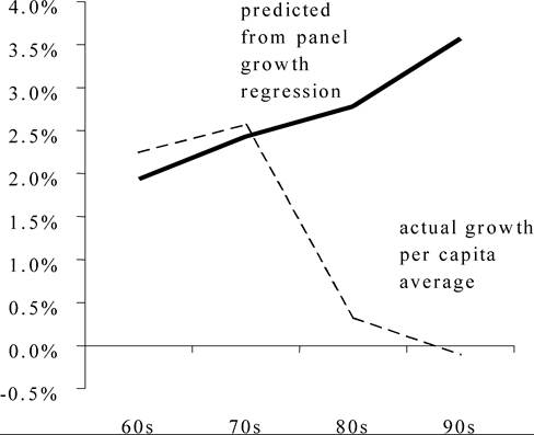
Figure 7. Predicted vs actual per capita growth for developing countries (assuming constant intercept across decades).
in determining development outcomes can only be limited. A view of economic development that puts all the weight on the 1960-2000 period is ahistorical, assuming away the complex histories of civilizations, conquests, and colonies.
Third, there is the general fact that developing countries had higher growth rates in the period 1960-1979 than in the period 1980-2000. Yet most of the “Washington Consensus” policies were adopted only after 1980. In the pre-1980 days, there was much more of an emphasis on state intervention and import-substituting industrialization, as opposed to the free trade, “get the prices right” approach after 1980. This big fact does not augur well for a strong positive effect of “good policies” on growth, although the growth slowdown after 1980 could have other causes. Easterly (2001) showed the divergence between improving growth predicted by policies and actual growth outcomes across the 60s, 70s, 80s, and 90s (see Figure 7).
Fourth, there are many income differences within nations - between the sexes, between ethnic groups, and between regions - that cannot be explained by national economic policies. Easterly and Levine show that there are four ethnic-geographic clusters of counties with poverty rates above 35 percent in the US: (1) Counties in the West that have large proportions (>35%) of native Americans; (2) Counties along the Mexican border that have large proportions (>35%) of Hispanics; (3) Counties adjacent to the lower Mississippi river in Arkansas, Mississippi, and Louisiana and in the “black belt” of Alabama, all of which have large proportions of blacks (>35%); (4) Virtually all-white counties in the mountains of eastern Kentucky. The county data did not pick up the well-known inner-city form of poverty, mainly among blacks, because counties that include inner cities also include rich suburbs. An inner city zip code in DC, College Heights in Anacostia, has only one-fifth of the income of a rich zip code (20816) in Bethesda MD. This has an ethnic dimension again since College Heights is 96 percent black and the rich zip code in Bethesda is 96 percent white. The purely ethnic differentials in the US are well known. Blacks earn 41 percent less than whites; Native Americans earn 36 percent less; Hispanics earn 31 percent less; Asians earn 16 percent more.[594] There are also more subtle ethnic earnings differentials.
Third- generation immigrants with Austrian grandparents had 20 percent higher wages in 1980 than third-generation immigrants with Belgian grandparents [Borjas (1992)]. Among Native Americans, the Iroquois earn almost twice the median household income of the Sioux. Other ethnic differentials appear by religion. Episcopalians earn 31% more income than Methodists [Kosmin and Lachman (1993), p. 260]. Twenty-three percent of the Forbes 400 richest Americans are Jewish, although only two percent of the US population is Jewish [Lipset (1996)].[595]Poverty areas exist in many countries: northeast Brazil, southern Italy, Chiapas in Mexico, Balochistan in Pakistan, and the Atlantic provinces in Canada. Bouillon, Legovini and Lustig (2003) find that there is a negative Chiapas effect in Mexican household income data, and that this effect has gotten worse over time. Households in the poor region of Tangail/Jamalpur in Bangladesh earned less than identical households in the better off region of Dhaka [Ravallion and Wodon (1998)]. Ravallion and Jalan (1996) and Jalan and Ravallion (1997) likewise found that households in poor counties in southwest China earned less than households with identical human capital and other characteristics in rich Guangdong Province.
In Latin America, the main ethnic divide is between indigenous and non-indigenous populations and between white, mestizo, and black populations. In Mexico, 80.6 percent of the indigenous population is below the poverty line, while only 18 percent of the non- indigenous population is below the poverty line.[596] But even within indigenous groups in Latin America, there are ethnic differentials. There are 4 main language groups among Guatemala’s indigenous population. Patrinos (1997) shows that the Quiche-speaking indigenous groups in Guatemala earn 22 percent less on average than Kekchi-speaking groups.
In Africa, there are widespread anecdotes about income differentials between ethnic groups, but little hard data.
The one exception is South Africa. South African whitescorrelation across sucessive 5-year periods for growth and policy variables
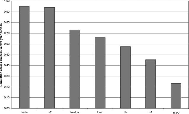
Figure 8. Persistence over time of policies and growth.
have 9.5 times the income of blacks. More surprisingly, among all-black traditional authorities (an administrative unit something like a village) in the state of KwaZulu- Natal, the ratio of the richest traditional authority to the poorest is 54 [Klitgaard and Fitschen (1997)]. While not ruling out national policy effects, these differences also highlight the importance of factors that do not operate at the national level.
Fifth, the role of policies in explaining post-1960 growth is bounded once we realize that policy variables are much more stable over time than are growth rates.[597] Figure 8 shows the correlation coefficient across successive 5-year periods between different kinds of policies and growth. As noted in the theoretical section, stability of policies over time and instability of growth rates is inconsistent with the AK model. It could be consistent with either the neoclassical model or the increasing returns growth model, assuming that policies are close to the steady state or critical point, respectively. Note that the non-persistence of growth rates and the high persistence of income levels is consistent, since persistent differences in growth rates would be required to scramble the income rankings from 1960 to 1999.
4. New empirical work
I here synthesize past results by running new regressions on an updated dataset for the years 1960-2000, using a panel of five year averages. Following the literature, I con-
Table 1
Variables used in analysis
| Variable name | Definition | Source |
| LGDPG | Log per capita growth rate | World Bank (2002) |
| INFL | Log (1 + inflation rate) | World Bank (2002) |
| BB | Government budget balance/GDP | World Bank (2002) |
| M2 | M2∕GDP | World Bank (2002) |
| LREALOVR | Log (overvaluation index/100)(above zero indicates overvaluation) | World Bank (2002) |
| LBMP | Log (1 + black market premium on foreign exchange) | World Bank (2002) |
| TRADE | (Exports+Imports)∕GDP | World Bank (2002) |
| GOVC | Government consumption/GDP | World Bank (2002) |
| PRIV | Private sector credit/total credit | World Bank (2002) |
| LNEWGDP | Log of per capita GDP | Summers and Heston (1991) updated using LGDPG |
| LTYR | Log of total schooling years | Barro and Lee (2000) |
centrate on the most common measures of macroeconomic policies, price distortions, financial development, and trade openness.
My variables are listed in Table 1.Table 2 shows the variables’ summary statistics.
Table 3 shows the correlation coefficients between these variables and growth as well as between distinct policies. All of the bivariate correlations of policy variables with per capita growth are statistically significant at the 5 percent level. Most of the pairwise correlations between policy variables are also statistically significant, indicating the problem of collinearity that has plagued the literature. Bad policies tend to go together along a number of dimensions. M2 and PRIV have such a high correlation that it is clear they are measuring the same thing - the overall level of financial development.
Table 2
Summary statistics
| Variable | Number of observations | Mean | Standard deviation | Min | Max |
| INFL | 967 | 0.159 | 0.325 | -0.569 | bgcolor=white>3.447|
| LNEWGDP | 921 | 8.107 | 1.040 | 5.775 | 10.445 |
| LGDPG | 1306 | 0.017 | 0.051 | -0.736 | 0.276 |
| GOVC | 1241 | 15.790 | 6.700 | 3.915 | 58.310 |
| BB | 958 | -0.037 | 0.054 | -0.417 | 0.391 |
| M2 | 1064 | 0.349 | 0.253 | 0.009 | 1.929 |
| PRIV | 916 | 0.355 | 0.329 | 0.000 | 2.085 |
| LREALOVR | 609 | 0.060 | 0.387 | -1.206 | 1.612 |
| LBMP | 1024 | 0.254 | 0.558 | -1.058 | 8.311 |
| Trade | 1270 | 0.702 | 0.454 | 0.018 | 3.803 |
| LTYR | 832 | 1.277 | 0.820 | -2.453 | 2.476 |
Table 3
Correlation coefficients
| LGDPG | INFL | BB | LREALOVR | LBMP | M2 | Trade | PRIV | GOVC | |
| LGDPG | 1.000 | -0.376 | 0.155 | -0.213 | -0.321 | 0.097 | 0.101 | 0.130 | -0.130 |
| INFL | -0.376 | 1.000 | -0.201 | 0.078 | 0.287 | -0.193 | -0.078 | -0.212 | 0.031 |
| BB | 0.155 | -0.201 | 1.000 | -0.141 | -0.144 | -0.010 | 0.094 | 0.110 | -0.231 |
| LREALOVR | -0.213 | 0.078 | -0.141 | 1.000 | 0.247 | -0.083 | -0.056 | -0.028 | 0.228 |
| LBMP | -0.321 | 0.287 | -0.144 | 0.247 | 1.000 | -0.073 | -0.178 | -0.241 | -0.036 |
| M2 | 0.097 | -0.193 | -0.010 | -0.083 | -0.073 | 1.000 | 0.375 | 0.716 | 0.246 |
| Trade | 0.101 | -0.078 | 0.094 | -0.056 | -0.178 | 0.375 | 1.000 | 0.161 | 0.276 |
| PRIV | 0.130 | -0.212 | 0.110 | -0.028 | -0.241 | 0.716 | 0.161 | 1.000 | 0.215 |
| GOVC | -0.130 | 0.031 | -0.231 | 0.228 | -0.036 | 0.246 | 0.276 | 0.215 | 1.000 |
I now concentrate on a core set of six variables that seem to capture distinct dimensions of policy: inflation, budget balance, real overvaluation, black market premium, financial depth, and trade openness.
Initially, I will test the AK model’s prediction that these policies will have growth rather than level effects, so I do not control for initial income (I will check this later on). I will use a variety of specifications and econometric methods to assess how robust are the statistical associations between policies and growth.I start off with a figure emphasizing the bivariate association between growth and different policies (Figure 9). I divide the sample into two parts, picking out the minority part of the sample where policy is extremely bad and comparing it to the rest (for inflation, black market premium, real overvaluation, and budget balance). Inflation, black market premium, and budget balance all have a distribution featuring a long tail of extreme “bad policy”, which seems like a real world experiment worth investigating. So I eyeball the distribution and pick a threshold that picks out this tail of bad policy.
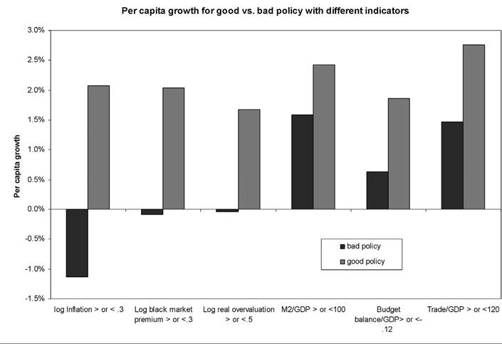
Figure 9. Bivariate effects of policy on growth.
Trade/GDP and M2∕GDP have a long tail for extremely good policy, so I pick a threshold picking out the extremes of good policy (see Figures 10-15). Real overvaluation does not have a long tail in one direction or the other, but I follow the same practice as with inflation, black market premium, and budget balance in setting a threshold that picks out extremely bad policy. Figure 9 shows that these experiments of either extremely good or extremely bad policy are associated with important growth differences. All of the differences are statistically significant except for the results on M2∕GDP Such strong associations have contributed to the conventional wisdom that policy has strong growth effects.
In Table 4, I regress growth on all six policy variables, and then try dropping one at a time. In the base specification, four of the six policies are statistically significant at the 5 percent level, with trade openness just barely falling short. When I experiment with dropping one variable at a time, all of the six policy variables are significant at one time or another. The coefficients on the policy variables are fairly stable across different permutations of the variables.[598]
Table 5 shows the effect on growth of a one standard deviation improvement in each of the policy variables on growth. If all six variables were improved at the same time,
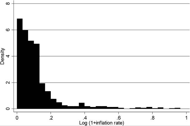
Figure 10. Histogram of inflation (truncated between 0 and 1).
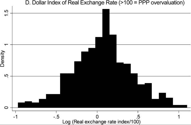
Figure 11. Histogram of real overvaluation (truncated between —1 and 1).
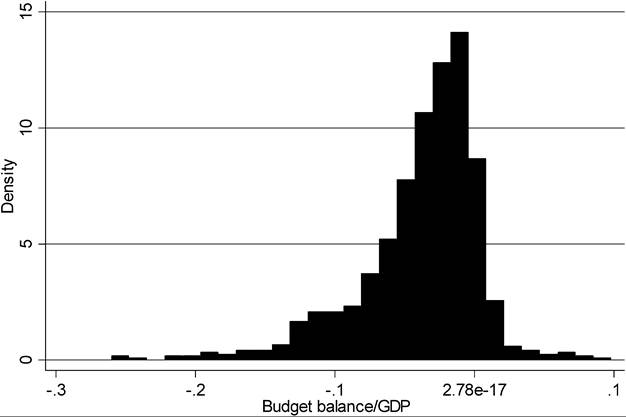
Figure 12. Histogram of budget balance/GDP.
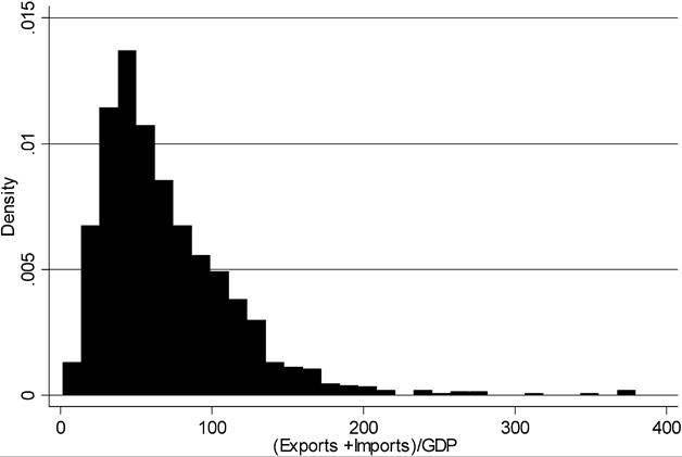
Figure 13. Histogram of trade/GDP (percent).
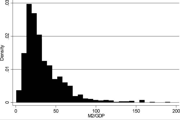
Figure 14. Histogram of M2∕GDP (percent).
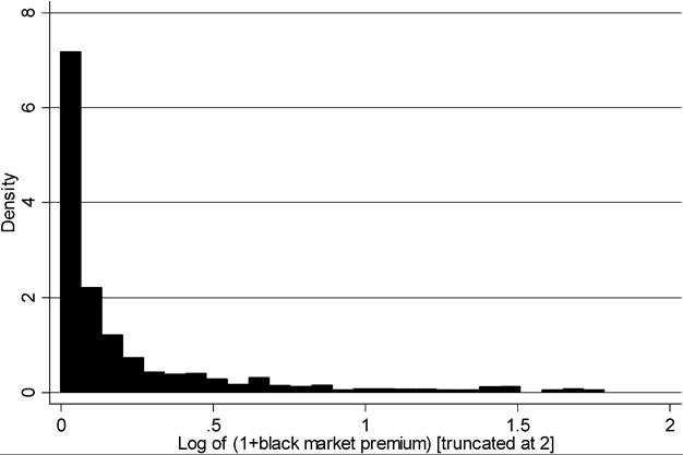
Figure 15. Histogram of Log of (1 + black market premium).
Table 4
Regressions of per capita growth on basic set of 6 policy variables. Dependent variable: LGDPG (log per capita growth, five year averages, 1960-2000)
| INFL | -0.018 | -0.02 | -0.02 | -0.034 | -0.021 | -0.018 | |
| (2.61)** | (3.13)** | (2.87)** | (6.27)** | (3.39)** | (2.60)** | ||
| BB | 0.092 | 0.114 | 0.092 | 0.053 | 0.109 | 0.098 | |
| (2.81)** | (3.48)** | (3.07)** | (3.07)** | (3.37)** | (2.92)** | ||
| M2 | 0.01 | 0.013 | 0.014 | 0.017 | 0.013 | 0.015 | |
| 1.37 | 1.92 | (2.04)* | (2.26)* | (1.99)* | (2.15)* | ||
| LREALOVR | -0.014 | -0.013 | -0.016 | -0.013 | -0.015 | -0.013 | |
| (2.97)** | (2.98)** | (3.74)** | (2.83)** | (3.56)** | (2.88)** | ||
| LBMP | -0.012 | -0.017 | -0.01 | -0.014 | -0.005 | -0.013 | |
| (2.33)* | (3.43)* | (2.06)* | (2.73)** | -0.93 | (2.60)** | ||
| Trade | 0.01 | 0.011 | 0.011 | 0.012 | 0.001 | 0.008 | |
| 1.92 | (2.22)* | (2.15)* | (2.62)** | 0.31 | (2.13)* | ||
| Constant | 0.016 | 0.013 | 0.01 | 0.021 | 0.019 | 0.015 | 0.021 |
| (3.62)** | (3.09)** | (2.33)* | (5.67)** | (4.81)** | (3.92)** | (5.55)** | |
| Observations | 422 | 434 | 458 | 495 | 573 | 455 | 424 |
| R-squared | 0.18 | 0.15 | 0.16 | 0.17 | 0.13 | 0.17 | 0.17 |
Robust standard errors, significant t statistics in parentheses.
* Significant at 5%.
**Significant at 1%.
Table 5
Effect of one standard deviation improvement in each policy variable on economic growth
| Variable | Improvement of one standard deviation in policy variable | Coefficient in growth regression | Change in growth from one standard deviation change in policy (%) |
| INFL | -0.325 | -0.018 | 0.6 |
| BB | 0.054 | 0.092 | 0.5 |
| M2 | 0.253 | 0.010 | 0.3 |
| LREALOVR | -0.387 | -0.014 | 0.5 |
| LBMP | -0.558 | -0.012 | 0.7 |
| Trade | 0.454 | 0.010 | 0.5 |
| Sum | 3.0 |
the regression suggests a 3 percentage point improvement in per capita growth. These results also seem to support the assertion that policies have strong effects on per capita growth.
The promise of getting 3 additional percentage points of growth due to a moderate policy reform package is very seductive. However, there is something disquieting about these results upon further reflection. The one standard deviation change in the policy variables is often very large: reduction of 0.32 in log inflation, 5 percentage point improvement in the budget balance as a ratio to GDP, 25 percentage point increase in M2∕GDP, reduction of -0.39 in log real overvaluation, reduction of -0.56 in log black market premium, and increase of 45 percentage points in trade∕GDP ratio. Such large changes are outside the experience of most countries with moderate inflation, budget deficits, real overvaluation, black market premiums, etc.
The large standard deviations are related to the long tails I mentioned above. Except for the real overvaluation index, all of the policy variables are highly skewed, with most of the sample concentrated at low values and a few very extreme observations. The outlying observations of inflation, budget deficits, and black market premium are realizations of extreme “bad policies”. The outlying observations of trade∕GDP and M2∕GDP are realizations of extreme “good policies”. It is econometric commonsense that extreme observations can be very influential in determining statistical significance of right-hand side variables. How do the above regressions do over more moderate ranges of policy variables?
Table 6 shows the effect of restricting the sample to observations where all six policy variables lie in the range of “moderate” policies. Moderate is defined rather arbitrarily by eye-balling the histograms above to determine where are the cutoffs containing the bulk of the sample (the same cutoffs as in Figure 9 above). Nevertheless, the cutoffs would fit a common-sense description of “extremes”: inflation and black market premiums more than 0.3 in log terms (35 percent), real overvaluation more than 0.5 (68 percent), budget deficits greater than 12 percent of GDP, M2 to GDP ratios of more than 100 percent, and trade to GDP ratios of more than 120 percent. The results of excluding any observation where any of the six policy variables are “extreme” is striking: all six policy variables become insignificant, and the F-statistic for their joint effect also falls short of significance. This is not to dismiss the evidence for policy effects on growth (reducing the range of the right-hand side variables would be expected to diminish statistical significance). These extremes are far from irrelevant, as observations in which at least one of the six policies was “extreme” account for more than half the sample. However, these results highlight the dependence of the policy and growth evidence on extreme observations of the policy variables. (The significance of extreme values and the insignificance of moderate ones is also consistent with the prediction of the theoretical model on the nonlinear effects of tax-cum-subsidy policies on economic growth.) There is also the possible endogeneity of these extreme policies, which may reflect general institutional or political chaos. The results suggest that countries not undergoing extreme values of these variables do not have strong reasons to expect growth effects of moderate changes in policies.[599]
Table 6
Robustness of results to restricting sample to moderate policy range. Dependent variable is LGDPG
| Sample | Full | Moderate policies |
| INFL | -0.018 | -0.064 |
| (2.61)** | -1.23 | |
| BB | 0.092 | 0.018 |
| (2.81)** | 0.22 | |
| M2 | 0.01 | -0.004 |
| 1.37 | 0.27 | |
| LREALOVR | -0.014 | 0.001 |
| (2.97)** | 0.06 | |
| Trade | 0.01 | 0.01 |
| 1.92 | 1.09 | |
| LBMP | -0.012 | -0.038 |
| (2.33)* | -0.95 | |
| Constant | 0.016 | 0.027 |
| (3.62)** | (2.52)* | |
| Observations | 422 | 193 |
| R-squared | 0.18 | 0.03 |
Robust t statistics in parentheses.
Restrictions under moderate policies: INFL between -0.05 and 0.3, BB between -0.12 and 0.02, M2 < 1.0, LREALOVR between -0.5 and 0.5, Trade < 1.20, LBMP between -0.05 and 0.3.
* Significant at 5%.
** Significant at 1%.
These results are fairly intuitive if we think of destroying growth as a different process from creating growth. It is a lot easier to cut down a tree than to grow one.[600] Countries that pursue destructive policies like high inflation, high black market premium, chronically high budget deficits and other signs of macroeconomic instability are plausible candidates to miss out on growth. However, it doesn’t follow that one can create growth with relative macroeconomic stability. The policies are inherently asymmetric - a leader can sow chaos by printing money and controlling the exchange until he gets a hyperinflation and an absurd black market premium. However, the best he can do in the other direction is zero inflation and zero black market premium. The results on policies and growth may simply reflect the potential for destruction from bad policies, not the potential for fostering long run development through good policy.
The only exception to this story is the trade/GDP variable, whose significance depended on “extremely good” policies. Whatever the source of the result on the extreme,
Table 7
Results on initial income and schooling
| Dependent variable | LGDPG | LGDPG | LGDPG | LGDPG |
| INFL | -0.018 | -0.019 | -0.02 | -0.019 |
| (2.61)** | (2.67)** | (2.65)** | (2.85)** | |
| BB | 0.092 | 0.102 | 0.124 | 0.107 |
| (2.81)** | (2.44)* | (2.65)** | (2.57)* | |
| M2 | 0.010 | 0.004 | 0.002 | 0.006 |
| 1.37 | 0.41 | 0.16 | 0.67 | |
| LREALOVR | -0.014 | -0.014 | -0.013 | -0.014 |
| (2.97)** | (3.07)** | (2.40)* | (2.96)** | |
| Trade | 0.01 | -0.01 | -0.01 | -0.011 |
| 1.92 | -1.83 | -1.63 | -1.96 | |
| LBMP | -0.012 | 0.01 | 0.008 | 0.009 |
| (2.33)* | 1.87 | 1.37 | 1.62 | |
| LNEWGDP | 0.003 | -0.001 | 0.0480 | |
| 1.4 | -0.28 | 1.96 | ||
| LTYR | 0.007 | |||
| 1.42 | ||||
| LNEWGDP2 | -0.0030 | |||
| -1.87 | ||||
| Constant | 0.016 | -0.004 | 0.019 | -0.187 |
| (3.62)** | -0.25 | -0.87 | -1.86 | |
| Observations | 422 | 411 | 359 | 411 |
| R-squared | 0.18 | 0.18 | 0.19 | 0.18 |
Robust t statistics in parentheses.
Turning point for convergence is 2981. *Significant at 5%.
** Significant at 1%.
this suggests that opening up for most economies - who likely would not reach this extreme even under complete free trade - would not be associated with growth effects.
The next thing to test is whether initial income belongs in the growth equation, as the neoclassical model would imply. It has also been common in the literature to add initial schooling as an indicator of whether the balance between physical and human capital is far from the optimal level. Table 7 shows the results on initial income and schooling.
The results are not very supportive of a conditional convergence result. Initial income and schooling do not enter significantly, although a nonlinear formulation of hump-shaped conditional convergence (including initial income squared) comes close to significance.[601] Since there is a large literature starting with Barro (1991) and Barro and Sala-i-Martin (1992) that does find conditional convergence, I do not claim this result
Table 8
Panel methods in policies and growth regressions. Dependent variable: LGDPG
| Panel method | Random effects | Between | Fixed effects |
| INFL | -0.019 | -0.012 | -0.02 |
| (3.53)** | -0.97 | (3.43)** | |
| BB | 0.082 | 0.216 | 0.069 |
| (2.35)* | (3.51)** | -1.64 | |
| M2 | 0.002 | 0.026 | -0.057 |
| -0.22 | (2.19)* | (3.16)** | |
| LREALOVR | -0.009 | -0.027 | 0.01 |
| -1.8 | (3.82)** | -1.43 | |
| Trade | 0.012 | 0 | 0.046 |
| -1.95 | -0.07 | (3.19)** | |
| LBMP | -0.011 | -0.01 | -0.012 |
| (2.15)* | -0.97 | -1.84 | |
| Constant | 0.017 | 0.019 | 0.016 |
| (3.22)** | (2.73)** | -1.61 | |
| Observations | 422 | 422 | 422 |
| Number of country units | 88 | 88 | 88 |
| R-squared | 0.17 | 0.41 | 0.13 |
| Sample | Full | Full | Full |
| Reject random effects | Yes |
Absolute value of z statistics in parentheses.
*Significant at 5%. ** Significant at 1%.
is decisive. It does show the fragility of the results on both policies and initial conditions (note that three of the policy variables become insignificant when initial income is included). I will come back to the issue of conditional convergence when I examine effects of policy on growth with dynamic panel methods.
There is another robustness check that we should perform on the policies and growth results. Following common practice in the literature, I have been doing regressions on pooled time series cross-section observations. This implicitly assumes that the effects on growth of a policy change over time are the same as a policy difference between countries. It is straightforward to test this restriction by doing within and between regressions on the pooled sample. Table 8 shows the results. I also show the results of a random effects regression, which gives results similar to OLS on the pooled sample. The test of whether the random effects are orthogonal to the right-hand side variables is an indirect test of the equality of the coefficients from the between and within regressions. I strongly reject the hypothesis that the random effects are orthogonal. We can see from the between and within (fixed effects) regressions that the coefficients across time and across countries are indeed very different. Inflation is not significant in the between regression but strongly significant in the within regression.[602] The budget balance is the reverse: strongly significant in the between regression but not in the fixed effects regression. The weak result that I found on M2∕GDP in the pooled regression turns out to be because the between and within effects tend to cancel out: M2∕GDP is strongly positively correlated with growth in the between regression and negatively correlated with growth in the within regressions. Real overvaluation and trade also show different results in the two different panel methods (real overvaluation is significant between countries and insignificant within countries, while trade is the reverse). This instability of growth effects is inconsistent with a simple AK view of growth with instantaneous transitional dynamics. It is also possible that five year averages are not long enough to wipe out cyclical fluctuations. The negative correlation between M2∕GDP and growth could be seen as a cyclical pattern such as a loosening of monetary policy during recessions and tightening during booms. Likewise the correlation of trade∕GDP with growth could indicate that international trade is pro-cyclical, as opposed to indicating any causal effect of openness on growth.
Also note that the r-squared of the between regression is much higher than the within regression. This is not surprising given that the between regression is on averages, but it does show that the growth effects of most concern to policy makers - the change over time within a given country of growth in response to policy changes - are very imprecisely estimated by the data. Fully 87 percent of the within country variance in growth rates is not explained by these six policy variables. This result is not surprising when we recall the persistence of policies over time and the non-persistence of growth rates.
Another panel method I apply to the data is the well-known dynamic panel estimator of Arellano and Bond (1991). This estimator uses first differences to remove the fixed effects. This method has several advantages: (1) it addresses reverse causality concerns by using twice-lagged values of the right-hand side variables as instruments for the first differences of RHS variables, (2) we can include initial income again, which is not possible with traditional panel methods because it would be correlated with the error term (Arellano and Bond address this by instrumenting for initial income with the twice- lagged value), and (3) we can also include the lagged growth rate to allow for partial adjustment of growth to policy changes, which is more plausible than instantaneous adjustment.
The results in Table 9 are notable in reinvigorating the conditional convergence hypothesis. This is consistent with previous work that shows a higher coefficient (in absolute value) on initial income with dynamic panel methods than with pooled or crosssection OLS [Caselli, Esquivel and Lefort (1996)]. The coefficient on lagged growth is not significant, failing to find support for the partial adjustment hypothesis. The results on policies are similar (not surprisingly) to the fixed effects estimator above. Inflation
Table 9
Regressions using Arellano and Bond dynamic panel method
| Dependent variable: LGDPG | (1) | (2) | (3) | (4) |
| LD.LGDPG | -0.0441 | -0.1131 | -0.09 | -0.0627 |
| (0.0749) | (0.0674)* | (0.0771) | (0.0823) | |
| D.INFL | -0.0137 | -0.0141 | -0.0162 | -0.017 |
| (0.0068)** | (0.0064)** | (0.0065)** | (0.0066)*** | |
| D.BB | 0.1014 | 0.0958 | 0.0876 | 0.0544 |
| (0.0509)** | (0.0501)* | (0.0540) | (0.0571) | |
| D.M2 | -0.0701 | -0.0457 | -0.0522 | -0.0486 |
| (0.0286)** | (0.0284) | (0.0302)* | (0.0307) | |
| D.LREALOVR | 0.0085 | 0.0081 | 0.0083 | 0.0021 |
| (0.0093) | (0.0087) | (0.0092) | (0.0098) | |
| D.LBMP | -0.0084 | -0.008 | -0.0037 | 0.0013 |
| (0.0086) | (0.0081) | (0.0086) | (0.0090) | |
| D.Trade | 0.0715 | 0.072 | 0.0635 | 0.0555 |
| (0.0201)*** | (0.0193)*** | (0.0204)*** | (0.0211)*** | |
| D.LNEWGDP | -0.0487 | -0.0508 | -0.0466 | |
| (0.0098)*** | (0.0104)*** | (0.0105)*** | ||
| D.LTYR | 0.0091 | 0.0137 | ||
| (0.0104) | (0.0105) | |||
| Constant | -0.0012 | 0.0014 | 0.0019 | 0.001 |
| (0.0016) | (0.0016) | (0.0020) | (0.0021) | |
| Observations | 323 | 316 | 275 | 275 |
| Number of country | 82 | 79 | 69 | 69 |
| Sargan | 36.51018 | 35.57537 | 31.19113 | 23.98194 |
| Prob > CHI2 | 0.0091 | 0.0119 | 0.0385 | 0.1968 |
| Test first order autocovariance | 0 | 0 | 0 | 0 |
| Test second order autocovariance | 0.9091 | 0.4666 | 0.5212 | 0.4797 |
| Time dummies | No | No | No | Yes |
Standard errors in parentheses. * Significant at 10%. **Significant at 5%.
*** Significant at 1%.
and trade are strongly significant with the right sign, while M2∕GDP still has a significant but perverse sign. The results do not change much if I experiment with omitting one policy variable at a time. The estimates are consistent because I fail to reject that second order serial correlation is zero. The difference with the fixed effects result on policies is that these results have somewhat more claim to being causal. However, the Sargan test rejects the overidentifying restrictions, except in the last equation where I add time dummies. This highlights a weakness of the strong claims for causality made by the dynamic panel method - they depend on the rather dubious assumption that the lagged right-hand side variables do not themselves enter the growth equation. The same problem afflicts the cross-section or pooled regressions that use lagged values of policy as instruments for current policies. Traditionalists who like intuitive arguments why instruments plausibly affect the independent but not the dependent variable are not very persuaded by lagged policies as instruments. As Mankiw (1995) noted sarcastically, if I instrument for the price of apples with the lagged price of apples in an equation for the quantity of apples, is it the supply or demand equation that I have identified?
6.
More on the topic Some empirical caveats:
- Some empirical caveats
- 7.7 The empirical meaning of differentiability
- Empirical studies of the effects of social capital
- Sustainable Value Added Tax (SVAT)
- Value and income
- Methodology
- DETERMINANTS OF LONG-RUN TRENDS IN INEQUALITY