DETERMINANTS OF LONG-RUN TRENDS IN INEQUALITY
How can we understand the trends in the distribution of income and wealth outlined in the previous sections? Do the series systematically relate to other developments in society that have been suggested to influence inequality, and if so, in what ways? How can we connect the observed long-run trends to existing theories about inequality? These are questions that we address in this section.
A number of facts that are likely to be important have already been noted in the previous sections along with the characterization of the trends. A first point is that an understanding of the development involves both wage and capital income, and thereby the dynamics are at least in part jointly determined by the distributions of income and wealth. For example, the drop in top shares over the first half of the twentieth century was largely a result of decreased capital incomes in the top, which in turn was largely driven by decreasing wealth shares in this group. High marginal tax rates in the decades after World War II made recovery difficult and caused top shares to decrease even further. We will explicitly look at these explanations in Section 7.4.2.
When it comes to the increase in top income shares since around 1980 this seems to be primarily related to increasing top wages, especially in the United States, but increasing capital incomes in the top also play a role in many countries (such as Sweden), especially after around 1990.1 4 The increased earnings dispersion is often attributed to aspects of globalization and technological change. Many have pointed to technological change being skill-biased, usually equated with an increasing education premium, as a possible reason for increasing wage differences. But skill-biased technological change does not
114
See Chapter 8 for a detailed view of inequality developments since 1970, where the increasing role of capital income in the top is also noted.
automatically lead to increasing wages of the “skilled.” The impact on wage dispersion depends on several things, such as the structure of the production function and the change in the supply of educated workers.[322] Unless the dynamics in “the race” between technology and education are made explicit, skill-biased technological change can be consistent with any number of “education premium” profiles over time.[323] Furthermore, even if one were to focus on a version of the model where the increased demand for skills actually lead to increasing wage dispersion, it is difficult to see how this would explain that so much of the increase is concentrated in a relatively small top group. To account for such increases within the top it seems necessary to find something that distinguishes a small fraction of the “skilled” from others who are equally educated (at least in terms of observables). Examples of such explanations include a number of so-called super-star theories, where technology and globalization disproportionately have benefitted those who—for various reasons—are most in demand in their field. Others have emphasized the possible role of changing norms. Some of the theories that have been put forth to understand the rise in top earnings over the past decades will be the subject of Section 7.4.3.
Finally, in Section 7.4.4 we present an overview of some recent econometric evidence on correlations over the long run. These regressions do not constitute tests of any particular theory but nevertheless give some insights as to what relationships seem to be present in the data.
We will begin the current section, however, with offering a broad overview of major events and societal trends that have been suggested to influence the distribution of income and how these correspond to our long-run pattern of top income shares. We will also discuss what the new series imply for our understanding of the Kuznets curve. Our conclusion is that, even if some broad trends are consistent with proposed broad explanations, we cannot distinguish between alternatives just based on looking at how inequality has developed.
Instead we need to look more carefully at developments in different parts of the distribution, at the source of income, and in particular on how income and wealth relate to each other and also relate all these aspects to predictions from theory.7.4.1 A First Look at Inequality Trends, Structural Changes, and Shocks What is the relationship between top income shares and the broad societal changes that have been hypothesized as affecting distributional outcomes? How well do the basic patterns match? Next we will discuss inequality developments in relation to trends in globalization, technological breakthroughs that have altered production in society (often referred to as general purpose technologies), inequality in relation to wars and shocks to the economy, and finally, inequality in relation to economic growth.
Globalization has been suggested to affect inequality in a number of ways. Classical trade theory in the spirit of Eli F. Heckscher and Bertil Ohlin has a clear prediction for inequality: In countries relatively abundant in skilled labor and capital (developed countries), inequality increases, whereas the reverse is true in (low-skill) labor abundant developing countries, where instead inequality goes down.[324] Modern trade theory is less clear-cut. Although some effects, like the gains to the largest most productive firms (in models like Melitz, 2003; Melitz and Ottaviano, 2008) seem to suggest increasing returns in the top, others have pointed to globalization being most beneficial for the top and the bottom, while hurting individuals in the middle of the distribution (e.g., Leamer, 2007; Venables, 2008). Yet others have pointed to the possibilities of efficiency gains from globalization being so large that these effects can compensate losses from, for instance, offshoring (Grossman and Rossi-Hansberg, 2008).
Looking at the inequality developments over what has been labeled as different waves of globalization, the first wave (1870—1914) coincides with flat or increasing inequality, followed by decreasing inequality in the antiglobalization period (1914-1950).[325] As most countries for which we have data belong to the relatively skill and capital abundant, this could be seen as in line with theoretical predictions.[326] The second wave of globalization is harder to reconcile.
In 1950-1980 measures of globalization (trade flows/ GDP, foreign capital as share of GDP) clearly increase while inequality clearly decreases. There are some obvious counterarguments to this. First, one may argue that the level of globalization was not yet sufficiently high for the predicted effects to show, but second, one could also point out that this was a period when most of capital flows and trade was between developed countries.1 0 Ifone places the start of the recent era of increased globalization around 1980 instead, the pattern is more promising as the period thereafter is characterized by increasing inequality. A problem is, of course, that during this period inequality has been increasing in developing countries too, counter to the basic Heckscher-Ohlin model.[327] [328]What about innovations leading to skill-biased technological change? Such shifts play a major role in the large literature trying to explain recent changes in the earnings distribution. Models building on Tinbergen’s (1974, 1975) seminal work suggest that the returns to skills are determined by a race between education (creating a supply of skilled workers) and technology (implicitly technology that complements skills). Technological change pushes in the direction of increased wage differences between skilled and unskilled, unless education keeps up and creates an increased supply of skilled workers that keeps down the wage differences. Goldin and Katz (2008) bring much of this work together in a unified framework. Acemoglu and Autor (2012, 2013) give overviews of much of this literature and also claim that these models have been empirically successful in accounting for recent wage dispersion mainly based on U.S. data (e.g., Autor et al., 2006; Katz and Autor, 1999; Katz and Murphy, 1992).
But, as already pointed out, skill-biased technological change does not automatically result in increased wage differences (and even less automatically in increased inequality).
Even in the simplest model the outcome depends on the speed of the supply response, and depending on the relative shifts in demand and supply of skills, the resulting wage differential between the groups can look different. In particular, this means that even if countries are affected by the same technological change, the impact on the wage distribution may look very different depending on how responsive countries are in terms of improving the skills in the population. See Atkinson (2008a,b) for more details and additional caveats to the simple model.[329]Another historical aspect of technological change, noted, for example, by Caselli (1999), is that it has not always been skill biased. Indeed, some of the technological advances in the late eighteenth and early nineteenth centuries replaced, rather than complemented, skilled artisans and increased the productivity of low-skilled workers (Mokyr, 1990). Later advances, such as the electrification of industry in the late nineteenth century, seem to have been more skill biased. Firms using more electricity paid workers higher wages, workers were more educated, and these firms had higher capital ratios (Goldin and Katz, 1998). But soon thereafter the introduction of the assembly line at Ford’s Highland Park facility in 1913 seems to be another technology shift that increased the relative productivity of unskilled workers.
If (and this is a potentially big “if”) one accepts that technology shifts that are skill biased always lead to increasing inequality, and vice versa for deskilling technological change, then the basic historical pattern looks promising. The skill-biased electrification coincides with increasing or at least unchanged inequality, the introduction of the assembly line coincides with the start of the long decline in inequality, and the recent ICT revolution starting in the 1970s and 1980s also happens at the time when inequality turns up again. But obviously this does not mean that we can conclude anything about the relationships.
In addition to the many assumptions needed, there are some other factors that are potentially problematic for a simplistic story of technological change driving common patterns of inequality. One is that technological changes do not take place everywhere at the same time. Comin and Mestieri (2013) give an overview of technology adoption lags and show that these can be very long. Second, given what we know about the role of capital in explaining the declining inequality in the first half of the twentieth century this seems separate from an explanation emphasizing returns to skills and an increasing earnings dispersion. Third, and perhaps most important, an explanation that focuses on the returns to higher education surely includes everyone in at least the top decile group. As such it cannot explain the large changes within the top and the fact that much of the recent increase has been limited to the income growth in the top percentile rather than a broader top group.Shocks in the form of wars and major financial crises constitute yet another broad category of explanations. As already noted in previous sections, these events certainly seem to have had an impact on top shares, especially in some countries, and in particular on capital incomes. The exact degree to which the equalizations following after the wars were due to outright destruction of capital owned by the wealthy or whether taxes and regulations redistributed wealth and increased overall socioeconomic mobility seem to have varied across countries. We discuss this issue further later.
Another broad topic concerns the relationship between inequality and economic growth. The crudest possible illustration of this could be done by dividing history since 1870 into four broad periods based on the overall inequality trends and calculating the average yearly growth rate over these. Starting in 1870 the average growth rate until today is 1.82% for the countries in the sample. Dividing this period into four subpe- riods—1870-1914, characterized by increasing (or unchanged) inequality; 1914-1950 characterized by rapidly decreasing inequality; 1950-1980, when inequality continued to decline but at a slower rate; and finally the period 1980-today, when inequality has been increasing—we can examine the average growth rate in each of these periods. It turns out that only one of these subperiods has an average growth rate higher than the long-run average 1.82%, namely 1950-1980, when average growth was 3.18%. This period is characterized by falling top income shares. The lowest growth rates are in the late 1800s and early 1900s when inequality was relatively flat (or rising), and growth rates in-between can be found both in the past 30 years 1980—2010 when inequality has increased, and in the period 1920-1950, when top shares declined. Based on this, it is certainly hard to see any clear secular (bivariate) relationship between inequality and growth.
7.4.1.1 What About the Kuznets Curve?
Despite Lindert’s (2000, p. 173) urge to the profession to “move onto explorations that proceed directly to the task of explaining any episodic movement, without bothering to relate it to the Kuznets curve,” we find it difficult to avoid discussing the Kuznets curve in this chapter. In the end we will, however, perhaps even more clearly thanks to the new evidence we have, come to the same conclusion.[330]
In its crudest interpretation, equating the Kuznets curve with the question, “Is it true that inequality first increases and then decreases as a country develops?” the answer must clearly be “No.” The fact that the broad pattern of decreasing inequality up until around 1980 has been followed by a sharp increase in some countries (but not all) clearly shows a pattern that is not consistent with inequality following an inverse U-shape, nor is it consistent with changes in inequality being the same across countries at similar levels of development. When testing the hypothesis on broad cross-country samples and in particular on developing countries, the evidence is mixed and inconclusive (Kanbur, 2000). With a broader interpretation it could be argued that increasing inequality in recent decades is, in fact, the start of a new Kuznets curve. The technological development starting in the 1970s constitutes the start of a shift, not from agriculture to industry as in Kuznets’ original story, but from traditional industry to an ICT-intensive sector that initially rewards a small part of the population, but eventually will spread, bringing inequality down. This idea would, under a number of assumptions, fit the general pattern better.
But even in its broader interpretation, a number of aspects do not fit the Kuznets curve hypothesis. First, when it comes to the first half of the twentieth century, a main finding of the recent top income literature is that most of the decline is a capital income phenomenon. Even if there was a continuous decline in the share of workers in agriculture and a large rural-urban migration, their impact on wage inequality was small; low- wage rural workers were mostly replaced by low-wage urban workers (see the discussion in Section 7.2.3.3 and also Piketty, 2006,2007). The inequality decline was, as evidenced by the timing of the fall, the source of income, and the concentration of the fall to the top percent group, due to shocks to wealth holders from the wars, the depression, and anticapital policies.[331] Second, the recent increase since around 1980 has the problem that it does not fit the predicted earnings dynamics within the distribution. As an increasing number become skilled, the difference within the top should decrease, not increase as seems to be the case.[332]
Taken together the preceding suggests that there is no mechanical relationship between inequality and industrialization or technological change. It is no more unavoidable that inequality increases at early stages of introducing new technology, than it is automatic that inequality eventually goes down. The Kuznets curve conjecture has indeed played an enormous role in shaping the research on long-run changes of inequality, but the recent research has made it even clearer that it is time to follow Linderfs (2000) suggestion to look at long-run changes “without bothering to relate it to the Kuznets curve.” In a way, part of the evidence suggests that other aspects also pointed to by Kuznets (1955) deserve more attention. After all, he formulated the famous Kuznets curve as a suggestion of how to explain what he saw as a puzzle of decreasing inequality. It was a puzzle because what he saw as the more obvious forces at play suggested that inequality be increasing in the countries he looked at: “There are at least two groups of forces in the long-term operation of developed countries that make for increasing inequality in the distribution of income...” ∣ Kuznets, 1955, p. 7). The first of these forces had to do with the interplay between the concentration of savings, the impact this would have over time on capital incomes, and income inequality. In forces that could counter such a mechanical increase of concentration he pointed to political decisions and taxation. These are all features that play a major role in potential explanations that we will look at in the next section.
7.4.2 Combining Wage Earnings and Wealth
The relationship between savings, income, and wealth discussed by Kuznets (1955) pointed to the need for a theory where individuals both work and receive income from capital, in different proportions. Such a theory was developed by Meade (1964). In his framework individual wealth holdings grow along with savings, s, and returns to capital, r, but diminishes across generations as the wealth is divided among a growing population that is 1 + n times larger in every period. If sr ≥ n wealth grows without limit but if sr < n then the division of wealth exceeds the growth of wealth, and wealth holdings converge to being a multiple of earnings.
Stiglitz (1969) embedded Meade’s framework in a general equilibrium model. Assuming that individual output is J(k), with k being capital per worker, a competitive rate of return, r, being the same for everyone and equal to J0 (k), and population grows at rate n, aggregate capital converges to a steady-state level where sJ(k)∕k = n. This in turn implies that sr < n so that in equilibrium division dominates growth of capital, and eventually the only thing determining wealth inequality is differences in earned income. This result, however, hinges on estates being divided equally. If one instead assumes that wealth is inherited by one child (as with primogeniture), so that wealth is not divided, long-run wealth inequality is compatible with the sr < n.
125
Furthermore, the resulting distribution will have a Pareto upper tail with Pareto coefficient α = ln (1n+1,+1”+t)), where sr(1 — t) is rate of accumulation out of wealth net of taxes, t (see Atkinson and Harrison, 1978, Chapter 8). This also suggests an empirical specification where we regress 1/a on sr(1 — t)/n.[333] However, even if primogeniture has been applied in the past (and still exists) the assumption of inheritance not being divided is implausible. In fact, today it is not even legal in most European countries. But there are several other assumptions that can be changed with the result that wealth inequality remains in equilibrium even if earnings are the same. Bourguignon (1981) shows that with a convex savings function there can be multiple locally stable equilibria, and with imperfect capital markets individuals with initially low wealth can be stuck in a “poverty trap.” Introducing stochastic elements allows for the possibility of escaping such a trap, but also introduces a new source of wealth inequality. Benhabib and Bisin (2007) showed how introducing an idiosyncratic rate of return results in a Pareto distribution for wealth that depends on capital income as well as inheritance taxes.[334]
Besides providing the first model to treat individual incomes as jointly determined by income and wealth, Meade (1964) also provided a basis for studying the joint impact of changes in wealth concentration and changing factor shares on the income distribution. To illustrate using the top percentile group, their share of total income can be broken down into one part based on earnings and one part originating from wealth holdings in the following manner:
Share of top percentile = (proportion of earned income) ? (share of top wage earnings percentile) ? (alignment coefficient for earnings) + (proportion of capital income) ? (share of top capital income percentile) ? (alignment coefficient for capital income). The alignment coefficient for earnings is the share in earnings of top percentile of income recipients divided by share of top percentile of wage earners and defined correspondingly for capital income. This captures the extent to which top wage earners and capital income recipients are also in the top of the total income distribution. In a class model where workers and capitalists are totally separate groups, there is zero alignment; workers have only earnings and capitalists only capital income. In a life cycle savings model with no inheritance, on the other hand, the same individuals inhabit the top of both earnings and capital income distributions, and the alignment is unity.
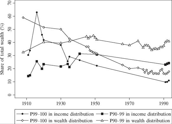
Figure 7.22 Wealth in top income and wealth fractiles in Sweden, 1908-2004. Notes and sources: See main text and Roine and Waldenstrom (2008) for further details.
Using this labor-capital decomposition it is, in principle, possible to attribute shifts in top income shares to shifts in top earnings shares, top capital income shares, and factor shares. A practical empirical problem, however, is that in most cases we lack data on the cross distributions over long periods oftime. Roine and Waldenstrom (2008), studying Sweden, is an exception. Thanks to a particular form of combined income and wealth tax it is possible to calculate the distribution of wealth ranked both by wealth and total income.1 8 Figure 7.22 shows that the share of total wealth when ranked by total income is somewhat lower than when ranked by wealth, but the two series are highly correlated, suggesting that there is significant overlap between the two distributions.
7.4.2.1 Explaining the Drop over the First Half of the Twentieth Century: Wealth Shocks and the Cumulative Effects of Taxes
Even if it is in most cases not possible to get a complete picture of the alignment of the distribution of earnings, capital income, and total income, a key feature of the top income data is the possibility to decompose income according to source. And, as already discussed in Section 7.2, it is clear that the drop in inequality in the first half of the twentieth century is mainly a capital income phenomenon. Combining what we know about the
128 Between 1910 and 1948 Sweden had a form of wealth tax according to which a share of individual wealth holdings (initially 1/60, later 1/100) was added onto other incomes. The tabulations of incomes therefore also contain wealth amounts by income groups. In addition, for a few years wealth and income tax data can be matched on an individual level.
composition of the drop according to income source (almost entirely capital income driven), the timing (in most countries concentrated to wartime and the Great Depression periods), and the development of wealth concentration (large decreases in wealth concentration), declining capital incomes among top earners constitute the main explanation for declining top shares.
It is interesting to note that this development came about even in counties not immediately exposed to all of the great shocks of the twentieth century. Sweden is a case in point. The world wars did affect the Swedish economy, but the country never participated directly in either of them, and looking at details in and around these periods it is clear that they did not constitute immediate shocks to Swedish wealth holders. If single events are to be pointed out, the economic crises in the early 1920s, the indirect effects of the GreatDepression, which hit Sweden in 1931, and, in particular, the dramatic collapse of the industrial empire controlled by the Swedish industrialist Ivar Kreuger (the “Kreuger Crash”) in 1932, stand out as being most important. These are, however, not sufficient to explain the drop in top shares in Sweden. Instead, a trend of decreasing share of capital in value added corresponds well to the declining top income shares. Policy, especially sharp increases in top tax rates, also stand out as important for explaining especially the drop just after the Second World War.
The general picture thus seems to be that macroshocks explain most of the drop, but there is also a role for a shift in policy and probably also in an economy-wide shift in the balance between returns to capital and labor.[335]
Assuming that we are satisfied with the explanation of why top shares dropped, we then face the challenge to explain why they did not recover in the decades after the Second World War, but rather continued to decline. Here a key factor seems to be the high rates of marginal taxation facing the top. The long-run evolution of statutory top marginal taxes is shown in Figure 7.23. As a broad generalization, top rates started to increase rapidly in the 1930s and reached high levels in many countries during and just after the Second World War.[336] As shown in Piketty (2001a,b, 2003), the combined effect of

Figure 7.23 Trends in top marginal tax rates, 1900-2006. SourcestSee main text.
shocks to capital holdings and high marginal tax rates is that recovery takes long. Unless adjustments to consumption are not made, current consumption levels can be sustained for some time by running down wealth holdings even further, but this decreases future income from wealth even more. An important point to note is that in these processes the short-run effect from taxes looks small. It is the cumulative effect over time that is
131
important.
How much do taxes impede capital accumulation and the recovery of top income shares? Just to illustrate the order of magnitude, assume a simple case with two groups of income earners; a top group that derives half their income from capital (the rate of return is assumed to be 5%) and the other half from wages, whereas the rest only have a wage income. Initially the income share of the top group is 15% of all income, and their consumption is such that their capital stock remains unchanged. These assumptions are, of course, not calibrated to fit any particular economy, but the numbers fit an approximate representation of the relationship between the top percentile and the rest of the population, both in terms of the importance of capital (with a broad interpretation) and the income share around World War II.
The combined effect of a tax increases from 30% to 60% and a shock that leaves the top group with 0.7 times initial wealth causes a gradual decline ofboth the capital income share (from 50% to 37% in 5 years and to 30% in 10 years) and total income share for the
131 Roine et al. (2009) also showed that the cumulative effects of the relatively small short-run impact of taxes found in their econometric analysis are consistent with much larger effects over time. top group (from 15 to 12.3 in 5 years, down to 11.1 in 10 years) with wages and consumption being unchanged. Despite the stylized nature of the setup, these magnitudes are reasonable when looking at data from the 1930s and following the Second World War. In the scenario with no changes to consumption wealth is eventually used up, and capital income goes to zero. Altering consumption too little makes the process longer but in the end the result is the same, whereas a sufficient adjustment allows for accumulation 132
over time.
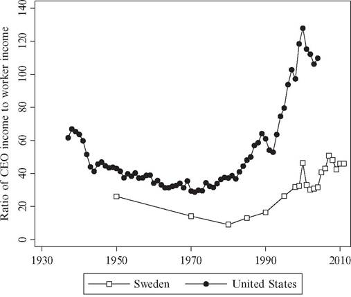
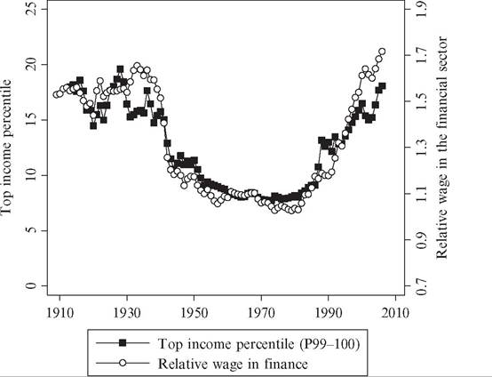
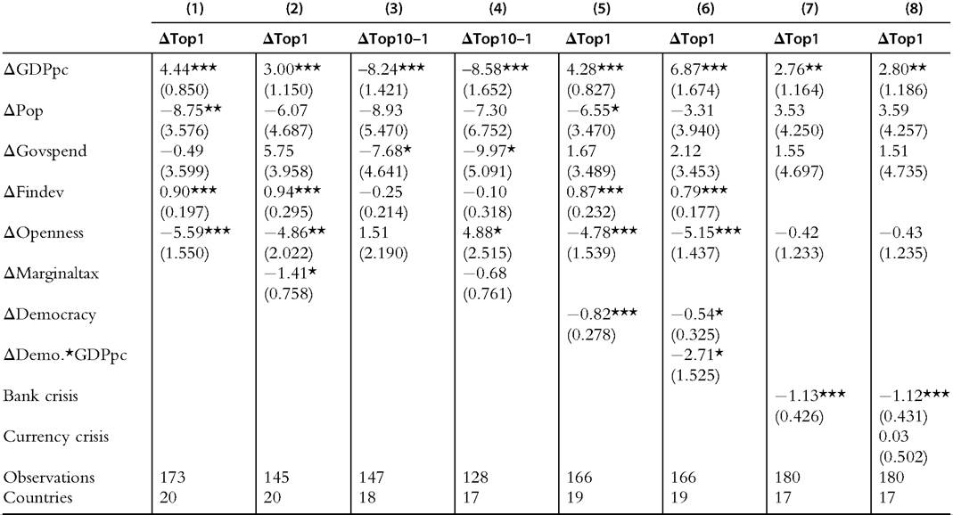
7.4.3 Explaining Increasing Top Wages: Executive Compensation, Superstar Effects, and the Possibility of Changing Norms
Although shocks to capital income combined with the cumulative impact of high marginal taxes are important in explaining the development between the First World War and around 1980, something else is needed to account for the increasing inequality since. This is especially true for understanding changes in top earnings, most visible in the United States, but also clear in many other countries (see Atkinson, 2008a, Chapter 4).[337] [338] As discussed in Section 7.4.1, it has been argued that increasing wage dispersion can be explained by theories of skill-biased technological change (Acemoglu and Autor, 2012, 2013) but also that these theories have some problems. In particular, it is hard to see how an increased advantage of the skilled, typically equated with the well-educated, squares with increased inequality not just in general but also increased inequality within the top group. There are several strands of literature that give insights into why the top of the earnings distribution may behave differently from the rest and what factors may govern compensation of top performers. This includes theories of determination of earnings in hierarchical organizations, tournament theory, and superstar effects. Research based on these ideas, and sometimes combinations of them, has tried to account for the sharp increase in top wages in recent decades. In models first developed by Simon (1957) and Lydall (1968) pay is related to the number of individuals supervised and to a (constant) pay increase at each step in the hierarchy. They assume that, first, at every level of the organization individuals supervise a constant number of people at the level below and, second, that the salary of these “managers” at every level is a constant proportion of the aggregate salaries of the people they directly supervise. More precisely, if at every level i of the organization there are yi employed, then the number of employed at the level below is γi~1 = syi. Furthermore, the wage wi at any level i is related to the aggregate of those below by a fixed proportion, p, such that wi = nwi 1p. Under these assumptions the upper tail of the earnings distribution log S 134 log (1+ p). will be approximately Pareto distributed with exponent α = the organization the people above will earn on average a constant of the wage at that level, the multiple being a/(a — 1). At any level in How much pay increases as one moves up in such an organization is determined by the number of individuals supervised and by the pay increase at every level, but also by the size of the organization. Iffirms become larger in terms of the total number of employees, the salaries of the top management can be expected to increase. This basic insight, that large firms pay their top managers more than small firms, was noted by Mayer (1960) and is also a prominent fact in the data on the distribution of CEO pay (see, e.g., the overview by Murphy, 1999). But the hierarchical models have other problems empirically, in particular when it comes to explaining the very top. As noted already by Phelps Brown (1977, p. 309) plausible values of the span of control (the number of direct subordinates at each level in the hierarchy) and the pay raise at each step of the hierarchy do not match observed Pareto exponents (see Atkinson, 2008a, p. 77). Individuals high up in organizations simply earn more than what the model would predict. In hierarchical models individuals are not paid based on “ability” but based on “responsibility.”[339] [340] But if “ability” determines the growth of a firm and the size of operations, then “responsibility” is endogenous, and the matching of ability and position becomes important.[341] In Rosen (1981) the distributions of firm size, span of control, and managerial incomes are modeled as the joint outcome of market assignments of personnel to hierarchical positions. Assuming the process assigns the most able individuals to the highest positions and that the talent of these individuals also multiplies throughout the organization, this results in firms of more capable managers being larger and also justifies high rewards to these managers.[342] In particular, it suggests that both the size distribution of firms and pay are skewed relative to the underlying ability distribution. Focusing on CEO pay across different firms, Tervio (2008) built on this kind of assignment model for managerial talent to a distribution of firms, where firm size may be different not just due to managerial ability but for other reasons as well. Under the assumption that the larger firms will have most to benefit from hiring the best managers, the pay levels of these individuals across firms will be determined by distributions of firm size and managerial talent. In such a context the value of the highest talent may be significant for the largest firm. In similar spirit, Gabaix and Landier (2008) suggested that even very small ability differences can have large impacts on firm value. They found the sixfold increase of U.S. CEO pay between 1980 and 2003 can be fully attributed to the sixfold increase in market capitalization of large companies during that period. A common feature in these (and many other) models is the idea that something (exogenous or endogenous) transforms small differences in the underlying ability to large differences in outcomes. Lazear and Rosen (1981) showed how compensation based on the outcome of a tournament where only the winner receives compensation can induce the highest effort under certain assumptions.[343] In general, attempts to implement payment schemes that give efforts to perform well has created a growth of performance-based pay in many fields. These schemes typically have the effect that the increase the individual returns to “top performers.” However, it is not clear that the effect is positive for the economy as a whole or even for the implementing firm.[344] In models following Rosen (1981) a combination of technological change (production that makes replication easier such as printing, recording) and the size of the market gives the “most talented” disproportionately large rewards.[345] As the market reach of a so-called “superstar” increases, the returns to the highest talent also goes up, and at the same time the returns to those just below in the ability distribution goes down. The “global leader” drives out individuals or firms that used to be competitive at a more local level leading to increased concentration in top rewards. Frank and Cook (1995) argued that an increasing number of markets have developed features that fit the superstar model; they have become what they call “winner-take-all-markets.” The examples range from activities where broadcasting in a wide sense enlarges the market (such as markets for sports stars, artists, writers), to those where hiring a “superstar” may become more important as the amounts that hinges on their performance grows (lawyers, investment bankers, and CEOs), to more standard product markets where decreasing transportation and other trading costs make increases the potential market.[346] So to what extent is the top of the distribution composed by such superstars? Kaplan and Rauh (2010) studied the representation of four sectors, top executives in nonfinancial firms, top employees in the financial sector (investment banks, hedge funds, and private equity), lawyers, and professional athletes and celebrities, in the top of the U.S. income distribution. They found that financial sector employees comprise a larger share than top executives from other sectors, and also that their share has grown in the past decades.[347] Athletes and celebrities as well as lawyers are certainly represented in the top but play a comparatively small role. Most striking perhaps is that the aggregate of these four groups account for less than 25% of the top income earners. This is due both to missing high- earning individuals in these four groups but also to the top of the income distribution consisting of much more than representatives of these groups. Overall, theories focusing on various ways in which the underlying ability distribution may be magnified in terms of top earnings certainly contribute to our understanding of the recent increase in top income shares. There are also a number of areas where it seems clear these effects have grown over the past decades. But also some developments suggest that these theories are unlikely to be the full explanation, especially if one looks at the longer run developments. Frydman and Saks (2007) studied the ratio of CEO to worker pay in the United States over the period 1936-2005. They showed that this ratio was falling between the 1930s and the 1970s even though firms certainly grew in size over this period. Over this longer period they concluded that relationship between pay and firm growth is weak. In Figure 7.24, we complement their U.S. data with corresponding data from Sweden for the period 1950-2011. The long-run picture is very similar with falling ratios until around 1980 and then clear upturns thereafter. The level difference between the countries is marked, however, as is the fact that the recent increase has been much larger in the United States than in Sweden. Another study that has looked at the long-run development of wages in a field with features that have been suggested to magnify small differences in ability, namely the financial sector, is Phillippon and Reshef (2012). They found that deregulation of financial markets is closely tied to compensation levels, as well as education levels and innovation, but also that the sector in the 1930s and since the 1990s seems to pay wages that are Figure 7.24 CEO and worker incomes in Sweden and the United States, 1936-2011. Note and sources: Ratios are based on the following series. U.S. CEO incomes in 2005 U.S. dollars refer to CEOs in the largest 500 corporations in the ExecuComp database, from Frydman and Saks (2007) (including salary, bonus, long-term payments, and options granted). This series was generously shared by Carola Frydman. Average income refers to workers in the Social Security Administration database, collected from Kopczuk et al. (2007, table A2, downloaded at http://www.columbia.edu/~wk2110/uncovering/, 201312). Swedish incomes refer to CEOs in the 50 largest Swedish corporations, and male industrial workers, data coming from LO (2013, bilaga 2, "Naringslivet"). substantially higher than what can be accounted for by observable factors (such as increased complexity of tasks and education levels). Interestingly, when comparing the relative pay in the financial sector with the top percentile income share in the entire United States, as is done in Figure 7.25, the resemblance is striking. The post-Depression drop in the 1930s is close to contemporaneous, and this is also true for the strong increase beginning in the late 1970s. Finally, some scholars have pointed to the possibility of changing social norms as the most likely explanation for why top earnings have increased so much in recent decades (e.g., Levy and Temin, 2007; Piketty and Saez, 2003). Atkinson (2008a, Chapter 8) illustrates how, in a setting where individual utility depends on income as well as conforming to a social norm about fair pay (which operates both on the employer and employee sides ofthe market), there can be multiple equilibria for a given distribution of underlying ability.[348] The loss of utility when not adhering to the norm depends on how many others do the same. As a consequence, market forces alone do not uniquely determine the 143 Figure 7.25 Relative wage in the financial Sectorversusthe top income percentile in the United States, 1909-2006. Note and sources: Ratio of financial sector wages to wages in agricultural and industrial sectors is from Phillippon and Reshef (2012) and U.S. top income share (excluding realized capital gains) are from Piketty and Saez (2003 and updates). outcome. There can be a situation where most individuals adhere to a norm, according to which pay is determined by a combination of ability and a fixed amount, as well as a situation where few individuals adhere to the norm, and pay is determined by individual productivity. Depending on initial conditions, different countries can converge on different pay norms, and “exogenous shocks” to the economy may cause a shift from one equilibrium to another. 7.4.4 Econometric Evidence on Determinants of Top Income Shares A key objective in the top income project has been to create a sufficiently rich cross-country panel to enable an econometric testing of questions about what determines inequality.[349] In this subsection we will report on the results from a number of such studies. 7.4.4.1 Determinants of Inequality: Correlations over the Long Run Roine et al. (2009) combined top income shares with data on a number of variables that have been suggested to affect inequality. The approach is not to test a particular theory but rather to draw on a large number of models to produce a list of variables of interest in an exploratory fashion (see Atkinson and Brandolini, 2006, for a discussion of the clear limitations with such an approach). Econometrically the adopted method is to analyze first differences (using both first differenced generalized least squares and dynamic (with lagged dependent variable) first differences), assuming a linear relationship at least in this specification. Panel estimations make it possible to account for all unobservable timeinvariant factors as well as common and country-specific trends. The potential that the relationships change over time is dealt with indirectly by allowing effects to differ over the level of development and for different country groups, and so on. This is clearly not the same as testing for the long-run effects of various variables on inequality but rather a way of testing what the short-run effects look like over the long run. The main variables included in the analysis are the following. Financial development is measured as the sum of stock market capitalization and total amount of bank deposits divided by GDP. Trade openness is measured either de facto as the trade share in GDP (i.e., sum of exports and imports over GDP) or de jure as the average tariff rate (total tariffs paid divided by traded volume). Public sector influence is proxied by the share of central government spending in GDP and as the top marginal tax rates. Finally, we also include GDP per capita and population.[350] Given the importance of changes within the top, the income shares of three groups are analyzed: the rich (P99-100), the upper middle class (P90-99), and the rest of the population (P0-P90).[351] Table 7.6 reports the regression results, and some basic relationships stand out as constantly robust across all specifications.[352] First, economic growth, that is, change in GDP per capita, seems to have been pro-rich over the twentieth century. In periods of faster than average growth, top income earners have benefited more than proportionally.[353] A likely reason for this result is simply that top incomes are (and have been) more closely related to performance than other incomes. This result is similar at different levels of Table 7.6 Long-run determinants of top income shares Notes: The regression methodandunderlyingdataare describedin Section 7.4.4.1 andRoine et al. (2009). “A” denotes log change between 5-yearperiods, “GDPpc” is real per capita GDP, “Pop” is population, “Govspend” is central government spendingas share ofGDP, “Findev” is the sum ofbanking deposits and stock market capitalization as share of GDP, “Openness” is trade share in GDP, “Marginaltax” is the statutory top marginal income tax rate, “Democracy” is the autocracy score in the Polity IV index, and “Bank crisis” and “Currency crisis” are dummy variables for years when such crises occurred. Robust standard errors in parentheses. *pthe capital stock and the effects of taxation. The recent increase in inequality, observable in many countries but not all, seems to be mainly due to increased top wages. Explaining this turns the focus to a different set of explanations emphasizing higher returns on the labor market for some groups (based on higher ability, skill, effort, education, etc.). Two key facts seem important in guiding efforts to understand this change. First, much of the increase is concentrated to a small fraction at the top of the population. This means that theories focusing on changes for broader groups (such as “skilled” and “unskilled”) at least need to be complemented by a mechanism explaining the increase within the top. Second, the degree to which top earnings have increased relative to the average is very different across countries. Thus, a theory based on a common global shift of some kind at least needs to be complemented with mechanisms that can account for the cross-country difference. Finally, the preliminary econometric evidence points to taxation being important in explaining the developments. Even though magnitudes in the short run may seem small, it is important to take the long-run dynamic effects into account. Financial development and economic growth being pro-rich also stand out as clear and robust correlates over the whole of the twentieth century, but so far we have only begun to use the data for systematic cross-country analysis. 7.5.