Value and income
Value and the resulting income are two fundamental output elements that are considered in financial analysis. All financial risk factors together with valuation rules affect value and income, which are the main drivers of both market and funding liquidity, as discussed in the previous sessions.
The results of income (positive or negative) are used as the basis in profit and loss analysis. Maximizing profit and optimizing risk are the main targets when defining the evolution in a new business production. Institutions employ both deterministic and stochastic approaches for measuring value and income at risk. The ratios of risk together with profit and loss measurements define the economic capital. Figure 12.4 illustrates all elements linked to value and income analysis.12.2.1 Estimating value
Actual and expected cash flow events include and drive the value and income of the financial contracts. As we have already seen above, the main input analysis elements that impact these cash flows are the market, counterparty and behavior risk factors. In measuring value, moreover, the applied valuation method plays a key role. We can illustrate the above by defining the value of fixed income financial contracts using the following Equation 12.5.

The indicator m defines the valuation method, NV (t) is the nominal value at time t and P∕Dm is a premium or discount function of NV based on valuation method m. The evolution of P∕D is linked to the notional cash flows (which also determine the nominal value) and their degree is derived by the risk-free market conditions, e.g., discounting the outstanding principals by referring to interest rates and calculating the interest payments that will finally adjust the initial value of the contract.
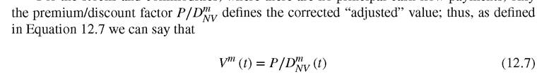
In a sense P∕D corrects the NV over time. Thus, at future time t, in fixed-income contract, the P∕Dm will derive the interest payments whereas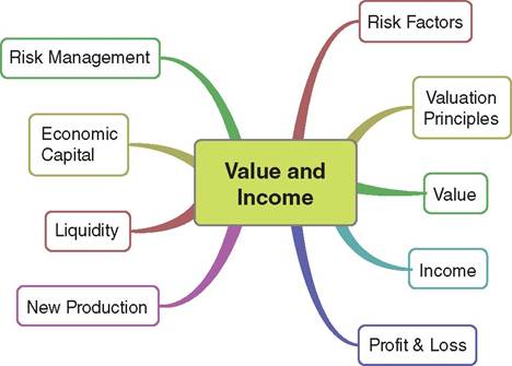
the nominal value NV (t) is derived by the principal cash flows CFp between t and maturity time as shown in Equation 12.6.

Therefore, nominal value is the base of any valuation concept which is, however, independent from valuation method. As aforementioned, nominal value is equal to the sum of outstanding principal payments, this definition becomes necessary if premium/discount is involved; on the other hand, interest payment cash flows are not involved in such value estimation.

In fact, for fixed income instruments, all valuation principles take into consideration the initial value (i.e., at value date), and the final value (i.e., at maturity date of the contract); they also define the path taken between these values through the time of the contract.
For the stocks and commodities, where there are no principal cash flow payments, only
In regards to off-balance sheet transactions, the aggregation of the underlying principal payments is equal to zero as they are balanced within the asset and liability positions, or the underlying contest is a forward transaction where the initial principal payment is balanced by the subsequent payments.
12.2.2 Estimating income
Income is derived by the changes of the above value over time considering the evolution of the financial risk factors as well as the valuation principle. Equation 12.8 illustrates the basic function of income.
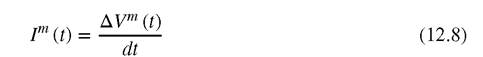
As we consider time the discretization of the above function could be usefully defined as illustrated in Equation 12.9.
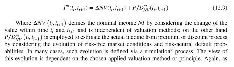
mentioned above, can be seen as the correction factor of the nominal income which depends on the valuation principle.
12.2.3 Profitandloss
Income is used to project the profit and loss analysis. Positive income indicates profit, whilst negative income indicates losses. Both positive and negative performance, together with the associated risk measurements, can be used to calculate the actual and expected returns as well as adjust the investment portfolio for resulting maximum profitability and minimum expected loss.
In profit and loss analysis all from existing past to simulated future value changes, positive and negative nominal income, the ΔP∕D values, as well as expenses or cost cash flows are registered and reported. The projection of future profits and losses together with the risk measurements are also used in the decisions of rolling over and/or constructing new portfolios, as will be discussed later.
12.2.4 Valuation principles
There are two types of valuation principles based on a) market dependent methods and b) time dependent or accrual methods. The former implies that the time evolution of P/D^iv depends mainly on market prices whereas in the latter the time evolution of P∕D'Nv does not depend on actual market conditions. The main time dependent principles are the nominal/write-off at the beginning, historic/write-off at the end, linear to maturity/reprising and amortized cost. Market dependent principles are the mark-to-market fair or observed values, lower of cost or market reflects the “principle of prudence” interpreted in a very strict manner. A full description of these rules is beyond the scope of this book; however, the reader can refer to the textbook Unified Financial Analysis.10
12.2.5 Risk on value and income
The main element that defines the value and income is the P∕D which is directly linked to the financial risk factors.
Any contract that is sensitive to changes and/or fluctuations of these factors during its lifetime will directly impact the corresponding value and income. The risk analysis is about identifying, measuring and managing these sensitivities over time. Risk is more related to “shaking” the real world rather than the risk-neutral expectations of markets and default probabilities as well as stressing the economic scenarios based on real-world probabilities as discussed in Chapters 6 and 7.Investors must be able to identify their strength as well as robustness against unexpected and extreme performance of the financial risk factors that their financial contracts are exposed to. They directly impact liquidity, value and income. Moreover there are many side effects, e.g. in the exposures to concentration and systemic risks. It is therefore very important that financial institutions are able to absorb any possible resulting losses due to unexpected real- world conditions but at the very same time are able to fulfil any other obligations against other counterparties that they may have. This will also imply that risk conditions will have the minimum impact on the entire market.
There are two important approaches11 in risk analysis: a) deterministically stressing and b) stochastically fluctuating the financial risk factors.
12.2.6 Stress testing
Deterministic scenarios can be applied for stressing at certain level(s) financial risk factor(s), in an individual or integrated manner, to measure the resulting unexpected losses. For instance, let's say a shock on an interest rate may be increased, within a quarter time horizon, up to 200bp whereas under such stress market condition counterparty(ies) are expected to downgrade one to two notches.
The assumptions of stress scenarios can be defined by the investor, the financial institution itself or by regulators and central banks. These assumptions can be driven by historical, current and future expected stressed market conditions.
Thus, historic models and what-if scenarios can be applied. Note, however, that history doesn't necessarily repeat itself and even if it does, not necessarily at the same cycles. Additionally, the current conditions do not remain steady whereas the future expectations may have several different paths. The problem becomes more complex as market risk factors usually interact with each other as well as with the other types of credit and behavioral risks. For instance, during a period of recession it is expected that interest rates will decline over time whereas some commodity prices may increase their values; moreover, due to market stress, borrowers may lose part of their strength to be able to fulfil the agreed credit obligations which indicates an increase of credit spreads.The definition of a scenario is a process looking from the past to future and defining meaningful stress conditions in a consistent manner. As markets are not static, stress conditions should also be applied considering also the evolution of these factors overtime.
12.2.7 Designing dynamic and integrated stress testing
Business is not static and there are existing contracts that may rollover after they mature; on the other hand, new contracts structure the production of new accounts and portfolios through time. The strategies on the evolution of new production must consider stress scenarios.
As mentioned, financial risk factors interact with each other; such interactions must be considered in the design of stress testing scenarios. Strategies also play a key role in stress testing. Table 12.2 illustrates a matrix of four different combinations that can be used to define an integrated stress testing scenario where both market conditions and counterparty status are considered in assumed (expected) stress cases. These obviously will drive the financial events,
TABLE 12.2 Combination of Market Conditions, Credit/Counterparty Status, behavior characteristics and new production in the design of stress testing
Credit/Counterparty Status
| Assumed | Stressed | |
| Market Conditions | Assumed Expected Financial Events (Expected Behaviors & Remained | Financial Events change due to Idiosyncratic Stress |
| Strategies) | (Stressed Behaviors / Reviewing | |
| Strategies) | ||
| Stressed Financial Events change due to new | Unexpected Financial Events | |
| Market Conditions | (Unexpected Behaviors & Change | |
| (Unexpected Behaviors & Reviewing Strategies) | of Strategies) |
the P&L as well as the behavior characteristics. Then, strategies and portfolios/accounts may be reviewed or restructured accordingly aligned with possible stress evolution of risk factors.
So, there are four main combinations that we could employ:■ The market conditions performing as assumed whereas there are no changes in counterparty credit status. In such case financial events appear as expected. Strategies may remain unchanged.
■ The market conditions are under stress whereas counterparty credit status is steady. Financial events are expected to change whereas strategies will be reviewed and possibly changed.
■ Market conditions are stable but counterparty credit status is under stress. Financial events will be changed due to counterparty idiosyncratic stress. Strategies should be reviewed and renewed.
■ Both market conditions and counterparties are under stress. Unexpected financial events will rise and strategies will be changed
12.2.8 Stochastic process
By using deterministic scenarios it is very difficult to cover all possible cases of real-world probabilities of the risk factors performances. Thus, stochastic process can also be applied to generate many different scenarios, which can be used to define a distribution of future values or prices of risk factors. As a result, the corresponding values of the portfolio con- tracts/instruments are obtained from such distributions which finally lead to the value distributions of the portfolio. This concept, defined as Value at Risk (VaR), has the scope to identify the notion of the maximum loss of a portfolio12 for a certain confidence level and pre-specified holding period.
There are different analytical and numerical methods for estimating VaR including Deltanormal, Delta-gamma, Parametric, Monte Carlo, Historical, Benchmark, etc. For instance, employing the very popular Monte Carlo approach, scenarios are generated for all risk factors in a random fashion, based on a variance-covariance matrix and a dynamic capital market model.
A more advanced approach is the dynamic VaR which is constructed based on the main market risk factors, a set of scenarios and strategies as well as the valuation concepts. The main additional feature of the dynamic Monte Carlo approach is the full integration of the time dimension. In contrast to the conventional static VaR, which has proven to be a consistent and reliable framework to measure short-term market risk, i.e., normally up to three months, the dynamic VaR methodology provides an answer to the market risk measurement problem when the relevant time horizon is long, from one to two years. While the static VaR consists in “instantaneous price shocks” of the market condition applied to the current balance sheet, the dynamic Monte Carlo method generates many market scenarios over a certain time horizon and simulates the activity of the financial institution over each of these scenarios. The relative impact in the income simulation, considering future strategies of the business evolution, can be used to measure the dynamic Income (or Earnings) at risk (usually denoted as IaR or EaR).
There is intense research and development of VaR approaches and relative systems and models implemented by both academia and the financial industry. Although there has been criticism of the stochastic process, especially during the crisis times, we should recognize the advantage of such approaches for considering a spectrum of risks and identifying as well as
measuring the degree of risk and resulting economic losses which lead to a definition of the corresponding economic capital.
12.2.9 Economic capital allocation and risk adjustments
Economic capital reflects the measurement of risks in terms of economic realities, i.e., scenarios, based on real-world probabilities, e.g., VaR calculation. Naturally, the measurement process involves converting a risk distribution to the amount of capital that is required to support the risk and absorb the resulting losses. The risk refers to both financial and operational instances. However, the former is more amenable than the latter. Economic capital provides a standardized unit measurement (i.e., a dollar of economic capital), and can become the basis for comparing and discussing opportunities and threats during the risk management process. As such, economic capital offers a language for pricing risk that is related directly to the principal concerns of strategies and profitability management.
The allocation of economic capital should be structured efficiently. Too little capital may not be able to absorb all losses; but setting aside a lot of capital, though safer, is costly. Thus, finding an optimal capital structure involves finding the right balance between the need for safety and the desire for maximizing return on capital. The idea is to assign capital charges to individual business and assigned portfolios based on their risk measurements. When risk-based capital allocation is used, the cost of managing (adjusting) the risks becomes a very important aspect. Such a method refers to the decision made on what type(s) of risk management should be applied, e.g., accepting, avoiding, hedging, transferring/mitigating. Risk is always linked to returns and available assets; therefore, a complete form of capital allocation should be driven according to the return on capital or assets and the ability of their risk adjustments. The general formula of risk adjustment is defined in the following Equation 12.10.

Using risk-adjusted performance measurement (RAPM) models, the risks and returns are compared against capital investments. The commonly used RAPM models13 are based on the return of capital (ROC) or return on assets (ROA). Risk-Adjusted Return on Capital (RAROC) is a model of RAPM, derived by the ROC function, which is mostly recognized by the financial industry. Equation 12.11 illustrates the RAROC function:

where the term performance, in the numerator, includes revenues but excludes expenses and expected losses and the risk in the denominator refers to capital reserves excluding, however, the ones referring to expected losses. A high degree of RAROC implies, therefore, a degree of risk, e.g., VaR, in relation to economic profit and vice versa. Consequently, a high degree of RAROC implies low requirements on a percentage (%) for the economic capital and vice versa. Thus, the ratio between economic capital and RAROC can be used to define the capital allocation as defined in Equation 12.12.

We could conclude therefore that combining risk measurements and profitability provides powerful and efficient ways to allocate capital against risk and unexpected losses and thus ensuring the stability of the portfolio through time.
12.2.10 Some key points in applying risk management
Finally, we would like to highlight that in the process of identifying risks the following characteristics should be considered:
■ An efficient degree of complexity. The selection of the approach and the identification and calculation of the risk measure should be simple but not simplistic. The degree of complexity for identifying, computing and reporting risk should be aligned with the complexity of the underlying risk factors and their integration.
■ Effectiveness, sensitivity and robustness. A small degree shock in the risk parameters that have been considered should cause not minor but rather significant impact to value, input, liquidity and relative losses. Moreover, risk measures must not be overly sensitive to modest parameters.
■ Transparency. All risk measurements should be available, explainable and understandable to the investors and the market participants.
■ Risk decomposition. The risk measurements should be decomposed within the responsible portfolios and linked to relative units and business lines. This will make the risk management simple and more applicable. This will also help in distributing and diversifying the effects of the corresponding losses as well as allocating the economic capital.
■ Consistency. The scenarios applied in risk factors must be consistent and provide coherent risk and profitability measurements, e.g., a stress of default probabilities should be aligned, and not in opposition, to stress credit spreads. Moreover, if for instance the impact to a portfolio A is less than in portfolio B then the latter is less risky than the former.
■ Intuitiveness. After all, even considering many risk factors driven by deterministic or stochastic scenarios the risk measure and reports should be meaningfully aligned somehow to the intuitive notion of the underlying real-world factors and probabilities.
■ Optimization. Risk management is about optimizing the portfolios to maximize profitability and minimize losses under economic scenarios based on real-world probabilities.
■ Cockpit. Just as a pilot in a cockpit does, a risk manager should be able to understand the exposures to different risks, where all relevant risk measurements are considered to ensure that businesses are running safely and profitably as well as ensuring that the system is robust in turbulent times.
■ New production. Risk management must always be linked to profitability analysis and strategies for restructuring the current, and planning the future, business. Thus, new production must always be linked to the evolution of parameters referring to risk and profitability.
12.3