LIQUIDITY
In a sense, a financial contract is a vehicle that carries and shifts cash flows among counterparties. However, too much available liquidity may cause investors additional exposure to risks such as interest rate and price volatilities.
Lack of liquidity implies frozen markets where investments cannot move further. The liquidity element is one of the most important analysis elements in finance. As long as cash is flowing as expected the market is performing at a stable status, any other case may cause high disturbances and great losses. When there is too much liquidity in the system, counterparties are in for a bumpy and volatile ride. Conversely, if liquidity freezes, counterparties are stuck without credit and need to wait until the ice thaws again.As liquidity refers to the past-to-future cash flows, time is a fundamental element in such analysis. There are two main types of generating cash flows, the contractual and the ones resulting from trading activities. The former is leading to funding and the latter to market liquidity analysis whereas their combination provides a full picture of liquidity risk. Moreover, it is the basis of defining the strategies on liquidity management for all types of existing and future development of new financial instruments including credit enhancements. Finally, reporting liquidity provides a strong overview of the cash flow management and precise warnings regarding survivor probabilities to liquidity risk. Figure 12.2 illustrates the main elements of liquidity analysis discussed in this chapter.
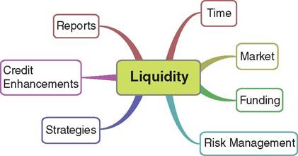
FIGURE 12.2 Main elements of market and funding liquidity and their risk management
12.1.1 Financial contracts and liquidity
The basic financial instruments provided, or traded, by banks, are fixed income maturity and non-maturity instruments, stocks, commodities and typical credit risk contracts.1 Basic instruments can be combined to create synthetic contracts such as swaps and forwards, futures, options, as well as credit risk derivatives, other structured securitization products, etc.
The expected cash flows for market participants result from the contractual payments, such as interest, principal, etc., but also from any financial trading activities due, for instance, to sales activities of liquid assets, driven by market expectations. The former refers to funding and the latter to market liquidity. It is also important to remember that the main cash flows from credit enhancements and other derivatives are expected when they are exercised, i.e., for hedging and covering losses.All expected cash flows depend on whether the counterparties are fulfilling their obligations and whether the market conditions and behavior risk factors are performing as expected. Thus, a default event will cancel out all expected cash flows whereas new cash flows will be generated due to credit enhancements and expected recoveries. The evolution of market conditions will affect the interest cash flows, and the values and prices of the financial instruments. At any time of trading, activities will generate immediate cash flows. Both market and counterparty driven behavior such as drawing, prepayments, recoveries, etc., will directly impact the expected liquidity.
The two main dimensions in liquidity analysis and reports are the time and the evolution of the business that will generate the cash flows. The main views of liquidity analysis are the funding and market liquidity. All are used to project the liquidity reports and identify whether the investment portfolios are producing the expected liquidity.
12.1.2 The time factor and types of analysis in liquidity
Inherently, the element of time is always considered in liquidity financial analysis, classified as liquidity horizon defining the time period when cash-flows returns will be considered, e.g., 90 days. As we will explain in the next paragraphs cash flows result from historical, static analysis and dynamic simulation.
In terms of liquidity, historical analysis is used to observe, from the view of a historic horizon, the actual cash flows generated up to the analysis (current) date; moreover, it is also important in back testing processes to examine how past market movements and counterparty status and behavior affected the liquidity of the actual cash flow events.
Static analysis examines the future expected cash flows based on the current and assumed performance of all financial risk factors linked to financial contracts, e.g., prices, discount factors, credit spreads, etc., at the current time of analysis. Current and assumed future conditions are considered to value the financial instruments and thus to identify their degree of liquidation in any possible trading activities.
Typically, the expected liquidity of the current investment portfolios and accounts are projected on so-called static views of:
■ Current positions and the up-to-date expected assumptions of market and economic conditions;
■ Current and expected credit status of the counterparty; and
■ Expected behavior risk factors.
Dynamic simulation is applied to consider the future evolution of cash flows based on the corresponding evolution of market conditions, counterparty status, behavior assumptions and future business. This implies future changes in the performance of the contracts, investment, trading of the portfolios and accounts through time. This is very much applied in the process of restructuring and building new future portfolios. Indeed, by keeping only the existing financial portfolios the size of investment will roll down as financial contracts mature. In reality, as time passes, new business usually generates growth in portfolios and accounts, whereby the future changing in financial risk factors must be considered.
Financial institutions and investors are applying dynamic simulation for the “goingconcern” view, based on new business analysis. In credit portfolios, new business means constructing new loans or rolling over the existing financial instruments. There is a strong link between new production and the projected market conditions, which enables forecasting of the performance of the future financial contracts. Thus, valuation, income and liquidity analysis should be based on the assumed future market and economic conditions and changes in credit spreads.
The production of new business is defined by an institution’s strategies, policies market/economic and credit risk conditions. This influences future portfolios and accounts and is usually a vital source of future cash flow to support cash out demands. Thus, it needs to be incorporated into the liquidity risk management framework.12.1.3 Market and funding liquidity risks
Liquidity risk can be thought of in terms of changes in expected contractual cash flows from the existing and future contracts as well as in traded financial contracts. These two initiatives of unexpected cash flows are called funding and market liquidity risks.
Market liquidity risk is about the inability of the financial institution to trade (sell or buy) financial assets of the favorable price at a requested time. For instance, due to unexpected price movements, higher bid-offer spreads and market impacts from trading, the revenues from the sale of assets may be less than expected (or the cost to purchase assets may be greater). Note that market liquidity risk is itself associated with market, counterparty credit and behavior risk factors that may transfer a liquid asset to illiquid; moreover, trading costs tend to be greatest when such factors are most volatile.
In fact market liquidity is very much contingent on the:
■ Performance of the financial risk factors
■ Strategic trading decisions e.g., for selling and/or buying liquid assets
The expected losses of this type of risk are estimated by comparing the estimated value of the assets under stressed conditions to their value in tranquil conditions. We therefore simply revaluate, let’s say, the fair price of financial instruments such as bond type, by discounting back the future cash flows taking into account economic scenarios based on real-world probabilities of market, credit and behavior stress risk conditions. Finally, note that asset-based credit enhancements that are exercised after default time can be heavily impacted by market liquidity risk.
Funding liquidity is about contractual obligations and management of contingent cash flows. Contractual cash flows are conditional on the pre-defined rules, options and algorithmic mechanics applied on the level of the individual financial contracts. Thus the expected cash flows,
■ For the loan contracts, i.e., from the obligor, are split into the following categories:
a. Principal payments defined at the contractual agreement (as illustrated in Chapter 5);
b. Interest payments (as illustrated in Chapter 5) which are derived by the market and credit conditions
■ For the stock and indices are due to expected dividends
■ For the derivative contracts are predefined premium payments, provided from the protection buyer to protection seller; also, in case of credit event, are the recoveries of financial losses
■ For the options have been agreed and may be exercised, e.g., prepayments, use of facilities, etc., cash flows may be generated.
Any unexpected changes of the above contractual cash flows—for instance, due to stressed market conditions, counterparty defaults, etc.—will result in unexpected cash flows incurring liquidity contingency issues and possible losses. This will possibly impact the value and thus market liquidity of the financial instruments.
Funding liquidity risk is about the inability of the counterparty to fulfil its contractual funding obligations under expected “normal” and unexpected “extreme” conditions. During normal financial risk conditions the demand for funding liquidity is usually steady. Under extreme conditions, however, some of the expected contractual cash flow: may be cancelled out (perhaps due to a default event), and/or resulted by exercising credit enhancements, or appear unexpectedly (for example, due to prepayments). Moreover, large market movements, for instance, may result in margin calls, changes in the degree of interest income, an increase of default probability, requests for additional collateral, etc. Naturally, there will be an impact on both liquidity and the value of such contracts.
In such cases financial institutions may be forced to sell additional liquid assets. To make matters worse, in this type of scenario the (normally) liquid instruments lose their value and may become illiquid,2 thus they are under market liquidity risk. That is, they cannot be traded quickly enough on the market, at a favorable price, to support liquidity demands or to prevent a loss. Finally, under funding distress the new expected business may shrink.Practitioners may apply a specific spread against market and funding liquidity risks. They also need to readjust3 their portfolios based on these types of risks.
In terms of analysis and measurement of liquidity risk, what-if scenarios may be applied for shifting the market conditions to a deterministic degree, whereas Monte Carlo methods may simulate stochastically the fluctuations of the markets, credit ratings, etc., to define the degree of resulting losses. Moreover, liquidity spreads may also be stressed. Thus, analysis due to unexpected conditions and resulting losses is the key element in both market and funding liquidity risk management. Finally, the behavior of sales, driven by idiosyncratic and strategic decisions, also plays a key role in market liquidity; for instance, structuring an inefficient credit portfolio or overselling particular assets may drop their value and turn them to an illiquid level.
In most analyses, funding and market liquidity are integrated due to their close connections. Market liquidity risk often leads to idiosyncratic funding liquidity risk and vice versa. In this context “idiosyncratic” refers to issues unique to the particular firm rather than market-wide liquidity issues. To map such integration, we need first to classify the analysis characteristics of both market and funding liquidity under normal and stress financial conditions and then analyze how and when they interact with each other as indicated in Table 12.1.
The first column/row of Table 12.1 refers to market and funding liquidity respectively; which, as discussed above, is driven by the impact of market and credit risks on value and
TABLE 12.1 Integration of Market and Funding Liquidity
| Funding Liquidity | |||
| Expected | Unexpected | ||
| Market Liquidity | Expected Risk | Case 1 | Case 2 |
| Factors Stressed Risk Factors | Case 3 | Case 4 | |
expected cash flows under normal and stressed conditions. Both static analysis and dynamic simulations can be applied, driven by current and future expectations, producing corresponding cash flows for liquidity analysis. For analyzing stressed conditions, deterministic or stochastic shocks can be applied to risk factors, including changes in spreads, to projected measures of market and funding liquidity risks. The shocks may relate to market/economic conditions as well as counterparty idiosyncratic characteristics.
The cases of combining funding and market liquidity risks where liquidity obligations and idiosyncratic liquidity funding management are integrated with the market value of the liquid assets can be summarized as follows:
■ Case 1: The parameters of market and funding liquidity are performing as expected. In this case, the exchange of cash flows resulting from the expected prices, discount factors, spreads, trading activities, credit losses, recoveries, etc. are as expected. Therefore, the liquidity funding process is supposed to be able to support the expected liquidity obligations.
Under normal, expected conditions, this is the most common case that markets and institutions have to deal with.
■ Case 2: Although the cash flows from the assets under market liquidity are as expected, the demand for liquidity outflows, from liabilities, is exceeding the expected degree and cannot be compensated for by the existing contractual inflows and liquidating process of liquid assets. In this case, the obligor is unable to fulfil the funding outflow liquidity obligations due to idiosyncratic inefficiency and/or distress.
Investors and obligors usually fall into this category due to inefficient structure of portfolio management lacking efficient liquidity management and thus may not be able to survive under stress conditions without external4 support.
■ Case 3: Market conditions may be under stress and thus liquid assets become illiquid resulting in minor and unfavorable cash flows. On the other hand the contractual cash flows from the existing portfolios provide the expected funding liquidity. The funding inflow liquidity may or may not be capable of overcoming the resulting loss, due to trading activities under market liquidity, and thus will be unable to fulfil possible additional cash flow requests and funding outflow obligations.5
Obligors facing such liquidity risk conditions may be able to survive during market liquidity turbulence due to their efficient portfolios and liquidity management as well as low idiosyncratic risk.
■ Case 4: The worst case scenario in terms of liquidity risk rises is when both market and funding liquidity are under stress, e.g., financial assets become illiquid and there are unexpected or cancelled contractual cash flows.
Obligors falling into this category—typically during a financial crisis—have little chance of surviving without external support.
Both investors and obligors must identify any combination of the above cases of market and funding liquidity risks. Institutions have a full range of liquidity risk management strategies and policies where contingency plans are in place for dealing with the extreme cases and liquidity needs.
12.1.4 Measuring and reporting liquidity and risk
The most applicable ways to measure the liquidity status are by projecting both contractual and tradable cash flows and identifying how long the obligor can survive without external support. The cash flow projections are reported via marginal liquidity gap reports whereas the liquidity survival period is estimated and reported via cumulative liquidity gaps.
The marginal liquidity gap is about considering all contractual and tradable cash inflows and outflows, aggregating them at the points in time defined through the cycle iteration (e.g., daily, weekly, monthly, etc.) of a predefined time bucket system, and making them visible in a single report. Thus, as shown in Equation 12.1, at each point in time ti the cash flows are aggregated within a time step i. Figure 12.3 illustrates a marginal liquidity gap report, where the single bars show the expected contractual net liquidity cash flows at a future time period. 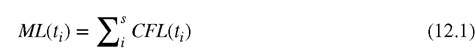
id="Picutre 126" class="lazyload" data-src="/files/uch_group74/uch_pgroup310/uch_uch7285/image/image126.jpg">
Cumulative liquidity gaps are based on marginal liquidity and are used to identify the time length of survivor period. Equation 12.2 shows the function for estimating such liquidity gap projection, where the cumulative liquidity CL at time tk is defined by aggregating the marginal liquidity cash flows. Cumulative liquidity reports are more intuitive and are extensively used in liquidity analysis.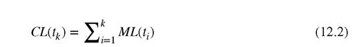
The liquidity survival period SP (t) within a liquidity horizon is defined as point at which the cumulative liquidity gap turns from a positive to a negative sign, i.e., the exact time when the cumulative liquidity will be equal to zero as illustrated in Figure 12.3.
Residual liquidity gap identifies the remaining cash flow position at a future point in time considering that no business will be renewed. The estimation of such a gap, as shown in Equation 12.3, is defined by considering the nominal value of the initial position at t0 minus the cumulative gap.

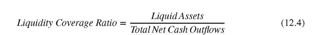
Based on market liquidity analysis the assets can be evaluated, and kept as a buffer, in regards to the level of their liquidation; on the other hand funding liquidity is about contracts cash in and out flows. Institutions assess6 their exposure to contingent liquidity events by calculating a liquidity coverage ratio. Such a ratio is equal to the stock of liquid assets,7 driven by market liquidity risk, over the total net cash outflows,8 and influenced by funding liquidity risk. Such a ratio must be over 100%. Equation 12.4 defines the general liquidity coverage ratio.
As already discussed, liquidity risk analysis is about integrating analysis of all financial risk factors which are not necessarily considered as risk-neutral but rather stressed into real- world probabilities. The key questions that we need to answer are the following:
■ What are the cash in and out flows during the lifetime of the contracts and the portfolio?
■ What is the maximum risk for losing liquidity survival period at a certain confidence level and liquidity horizon?
■ How much are we exposed to contingent liquidity events?
When financial risk factors are deterministically defined and may be stressed, the resulting cumulative liquidity gap will illustrate the liquidity survival period. Moreover, where that risk factor or factors have been historically changed or will be changed based on different (stochastic) scenarios over time, then we have a distribution of the resulting cumulative liquidity gaps which will illustrate the corresponding distribution of liquidity survival periods. Based on the distribution of liquidity survival periods the liquidity at risk (LaR) can be estimated. Under stress conditions the expected cash flows may be cancelled out and replaced with others; moreover, under market and/or funding liquidity risk the expected liquidity contingency may be under risk.
12.2