Volatility and growth: the AK approach

In an AK model where long-run growth is entirely driven by cap­ital accumulation, the average growth rate depends positively on the savings rate. The savings rate in turn is affected by the degree of macroeconomic volatility, however in a way which is a priori ambiguous: (i) increased volatility induces individuals to save more for precautionary reasons, which in turn leads to a higher equilibrium savings rate and therefore a higher average growth rate in this AK model; (ii) higher macroeconomic volatility tends to reduce the risk-adjusted returns on capital accumula­tion, and therefore individuals' incentives to sacrifice short-run consumption at the expense of investment; this latter effect tends to discourage savings and thus reduce the average growth rate.

Consider an economy populated by a continuum of individuals who live for an infinite number of periods, and share the same intertemporal utility function:

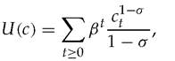
where β is the discount factor and

e = 1∕σ

is the intertemporal elasticity of substitution of a representative individual (equivalently, σ is her coefficient of relative risk­aversion). There is only one good in the economy, which serves both as capital and for consumption purposes.

In each period t, the representative individual produces final output using capital, according to the stochastic AK technology

yt = Autkt, (1.1)

where A is a productivity parameter which is invariant over time, ut is an aggregate multiplicative productivity shock with mean equal to 1, and kt is the capital input used to produce final output at date t.

In the initial period 0, the representative individual will choose how to divide final output between consumption and investment, by solving the intertemporal maximization program:

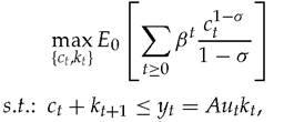
where Eq denotes the expectation, as of date 0, over all subsequent realizations of the aggregate productivity shock.

The first-order conditions for this maximization, can be expressed by the set of Euler equations:

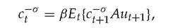
where E_t denotes the expectation over the realization of the pro­ductivity shock u_t at date t. We are supposed to solve this equation jointly with the budget constraint, c_t + k_t+1 ≤ Au_tk_t, to get to the optimal consumption rule.

To get to this solution, let us start with the guess that consump­tion is a fixed fraction of output:

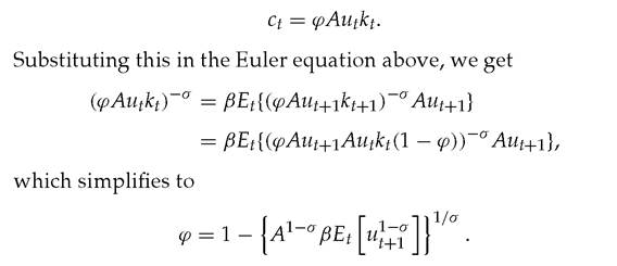
Since this is evidently a constant, we see that the linear con­sumption rule, c_t = φAu_tk_t, satisfies the first-order conditions for a maximum.¹

Given this consumption rule it is easily checked that the expec­ted growth rate of output from one period to the next will be given by

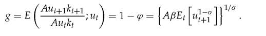
We are now able to address the question that this exercise poses: How does the average growth rate g, vary with macro­economic volatility?

It is easy to see that a mean-preserving spread in the distribu­tion of aggregate productivity shocks {u_t}, will increase growth if u^¹+σ is convex in u and reduce it otherwise.

1

It can be checked that this actually represents a global maximum.

whether the coefficient σ is greater or smaller than 1. Specifically if the intertemporal elasticity of substitution e = 1∕σ is greater than 1, then u^1-σ is concave and therefore an increase in volatil­ity reduces expected growth. In this case, the dominant effect of volatility is to reduce the risk-adjusted return on investment and thereby discourage savings. If instead, as appears to be the case from the available data,^[3] the intertemporal elasticity of substitu­tion is less than 1, then u^1-σ is convex and therefore volatility increases expected growth. In this case, the dominant effect of volatility is to increase precautionary savings and growth.

Thus, according to this AK approach, growth should increase with volatility for observed values of the intertemporal elasticity of substitution e.

1.2