The Schumpeterian approach

A second approach to volatility and growth emphasizes the dis­tinction between short-run capital investments and long-term productivity-enhancing investments. Examples of such long-term investments include R&D, IT equipment, and organizational cap­ital.

This “opportunity cost"argument was first spelled out by Hall (1991), who constructed a model where a constant labor force is allocated between production and the creation of organiza­tional capital (in contrast to real business cycle models where the choice of activities is between production and leisure). Hall writes, “Measured output may be low during [recession] periods, but the time spent reorganizing pays off in its contribution to future pro­ductivity." Subsequent work by Bean (1990), Gali and Hammour (1991), and Saint-Paul (1993) looked for empirical evidence sup­porting the existence of the opportunity cost effect.³

1.2.1 Basicframework

The following model is directly drawn from Aghion-Angeletos- Banerjee-Manova (AABM) (2004). Time is discrete and indexed by t. Suppose that at each date t, aggregate productivity A_t fluctuates around a benchmark level T_t which we refer to as the stock of knowledge at date t. We denote by a_t the ratio A_t/T_t: A low value of a_t corresponds to a bad productivity shock.

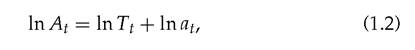
where a_t represents an exogenous productivity (or demand) shock in period t.⁴

There is a continuum of two-period lived entrepreneurs, which are all ex ante identical. Entrepreneurs are risk neutral and con­sume only in the last period of their lives. Each entrepreneur born in each period t has initial wealth (or human capital endowment equivalent to the amount of wealth) and this wealth is proportional

³ Using a VAR estimation method on a cross-OECD panel data set, Saint-Paul (1993) showed that the effect of demand fluctuations on productivity growth is stronger when demand fluctuations are more transitory.

⁴ As in RBC (Real Business Cycle) models, the shock is assumed to follow a random process of the form

where εt is normally distributed with mean equal to (—σ²/2) and variance equal to σ² (so that the expectation of the productivity level At is equal to the level of knowledge Tt). The parameters ρ ∈ [0,1) and σ > 0 measure respectively the persistence and volatility of the exogenous aggregate shock. Note that Tt can be interpreted as the "trend"in productivity. to the aggregate level of knowledge, T_t. Let w = Wt/Tt denote the (constant) knowledge-adjusted wealth of an individual at birth.

In the first period of his or her life, the entrepreneur must decide on how to allocate his or her initial wealth endowment between short-run capital investments, K_t, and long-term investments, Z_t. To ensure a balanced-growth path, we assume that, like for initial wealth, the costs of the two types of investments are also propor­tional to current knowledge T_t, and therefore the relevant variables in our model will be k_t = K_t/T_t, and z_t = Z_t/T_t, the knowledge- adjusted holdings of capital and R&D investments respectively.

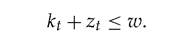
Short-run capital investment at date t generates income 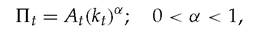at the end of the same period. Thus, in the short run, the entrepren­eur produces according to a completely standard Cobb-Douglas production technology with productivity parameter A_t.

The interesting part of the model comes from long-term invest­ments: Long-term investment at date t generates income at date t +1 only if the firm can meet some additional liquidity needs that arise at the end of period t. These costs arise either because the pro­ject itself needs some additional investments or because the owner of the firm needs to deal with some other problems before he is ready to realize the returns from his long-term investments. Thus, there may be a health crisis that needs to be dealt with before he can focus on the new project. Or there may be a problem in his estab­lished busines, which needs to be fixed before he can expect to do anything new. In all of these cases, he needs to spend additional money, the magnitude of which remains unknown until the end of period t. Like all other variables, this cost, C_t = c_tT_t, is assumed to be proportional to the current knowledge level T_t, and we denote by c_t the knowledge-adjusted liquidity needs of long-term invest­ment. The realization of this cost is uncertain at the point when the entrepreneur decides on how to allocate her wealth between short- and long-term investment.

The initial long-term investment pays off in period t + 1, but only if liquidity needs have been met. In this case the entrepreneur recoups her liquidity needs and, in addition, realizes the long-term profit in period t + 1:

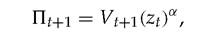
where q(z_t) = (z_t)^α is the probability that the long-term investment is successful and V_t+1 is the value of a new innovation (which we spell out below). If the entrepreneur can cover the liquidity needs of long-term investment, he or she innovates and recoups the cost, or he or she cannot meet that cost, in which case the productivity remains unchanged in period t + 1.

Now, we turn our attention to growth and the dynamics of knowledge over time. As in other models of endogenous tech­nical progress,^[4] only the long-term investments, z_t, contribute to long-run growth, with knowledge accumulating over time at a rate proportional to the aggregate rate of innovation in the economy. Namely:

where f_t denotes the fraction of entrepreneurs who manage to meet their liquidity needs. In this chapter, we assume perfect capital markets: It will turn out that therefore f_t = 1, since once you choose to invest in the long-term project, it always pays to meet the liquidity need. Note that the growth rate of knowledge as defined by (1.4), will certainly vary over time since, z_t, the amount of long­term investment itself fluctuates with the current realization of the productivity shock a_t (we shall see how in a moment).

This long-term investment may be thought of as R&D. However, it is probably more natural to think of it as the starting of a new line of business, or the introduction of a new technology, or the development of a new market.

1.2.2 The opportunity cost effect

and the knowledge-adjusted value of a new innovation in period t + 1. Our main assumption here will be that the returns to long-term investment are less procyclical than the return to cap­ital investments. This amounts to assuming that the correlation between v_t+ι = V_t+ι∕T_t and a_t = A_t∕T_t over the business cycle is less than one, which, in turn is necessarily the case as long as the productivity shock is less than fully persistent and the value of innovation represents a present value of returns over a horizon extending beyond period t.

which in turn implies that the expected knowledge-adjusted value of an innovation at date t + 1, is simply expressed as⁶:

In the absence of credit market imperfections, an entrepreneur will always be able to borrow what is necessary in order to cover his or her liquidity needs. This implies that the long-term investment of an entrepreneur in his or her first period of life will always pay out next period in the form of future revenues v_t+1 from innovating. More formally, consider an entrepreneur born at date t. Her final expected wealth at the end of period t + 1 is equal to

which the entrepreneur maximizes subject to her budget constraint Now, if we concentrate on interior solutions, we obtain the first- order conditions:

where λ is the Lagrange multiplier on the budget constraint.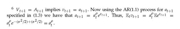

These conditions immediately imply that z_t is countercyclical whereas k_t is procyclical, with:

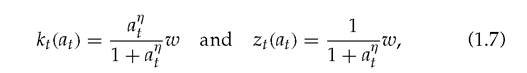
where η = (1 — ρ)∕(1 — α) > 0. The intuition is straightforward: Suppose there is a good productivity shock, that is, a high real­ization of a_t at date t. With such a high productivity level, it is more profitable to invest in short-run production than in long­term investment, which will improve productivity in some future period that will probably be less productive.

This countercyclicality, in turn, has important implications when analyzing the effect of volatility on growth. From the growth equation (1.4), the average growth rate of technology in the long run is equal to:

spread in a_t should translate into a higher expected growth rate g_t. The intuition for the result is shown in Figure 1.1, which pictures the equilibrium innovation probability (zt(a_t))^α as a function of a_t. We clearly see that the convexity of this function implies that a mean-preserving spread from perfect certainty over the real­ization of a_t, increases the average rate of growth-enhancing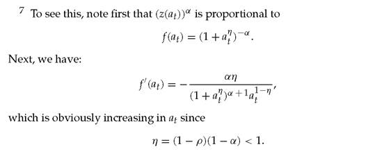

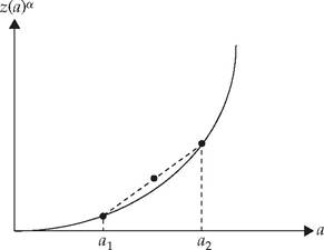
Fig. 1.1 Equilibrium innovation probability.

Note: If we randomize between ai and α2, the average innovation probability lies strictly above the curve.

investments. Thus, without credit constraints, this opportunity cost model of volatility and growth delivers again the prediction that higher volatility should translate in higher growth. As we shall see in the next section, in spite of the potential suggested above, which points to a potential positive effect of recessions on "organizational capital," the overall cross-country evidence on volatility and growth goes pretty much the other way.

1.3