Benefits and Costs of Higher Capital Requirements for Banks
This chapter provides new estimates of the likely economic losses from banking crises. It also provides new estimates of the economic cost of increasing bank capital requirements, based in part on the estimate in chapter 3 of the empirical magnitude of the Modigliani-Miller (M&M) effect in which higher capital reduces the unit cost of equity capital.
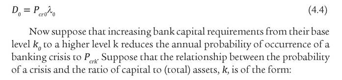
The study applies previous official estimates (BCBS 2010a) of the impact of higher capital on the probability of banking crises to derive a benefits curve for additional capital, which is highly nonlinear. It examines the benefit and cost curves to identify the socially optimal level of bank capital, which it estimates at about 7 percent of total assets (corresponding to about 12 percent of risk-weighted assets). A more cautious alternative (75th percentile across 2,187 possible outcomes under alternative parameter assumptions) places the optimum at about 8 percent of total assets, corresponding to about 14 percent of risk-weighted assets. These levels are, respectively, about one- fourth to one-half higher than the Basel III capital requirements for the large global systemically important banks (G-SIBs).Higher bank capital requirements reduce the probability of banking crises. Combining this reduction with estimates of the economic cost of banking crises provides a basis for calculating the “benefit” of higher capital requirements. This benefit is the expected damage avoided by reducing the risk of occurrence of a banking crisis. This chapter first quantifies the expected costs and frequency of banking crises, paying special attention to
An earlier version of this chapter appeared in Cline (2016a). The equations and quantitative estimates are unchanged. avoiding overstatement of recession losses if the economy has an unsustainable positive output gap prior to the crisis, as well as to finite life of losses considered to persist after the first few years of a crisis.
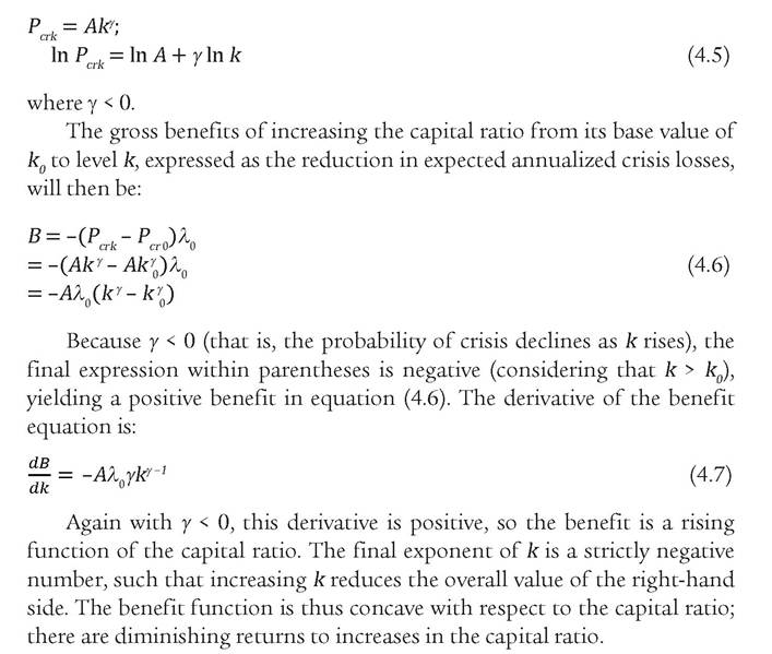
The benefits section then calibrates a “benefits curve” relating damages avoided to the level of bank capital, based on the most important official survey of the influence of bank capital on the likelihood of banking crises (BCBS 2010a).The analysis then turns to the cost curve relating economic costs to the level of the capital requirement. This relationship turns out to be an upward-sloping straight line. The cost line is steeper if the M&M offset is lower, the excess unit cost of equity versus debt is higher, there is spillover to nonbank finance, the capital share in output is higher, and the elasticity of substitution between capital and labor is higher. The optimal level of capital will then be the amount at which the slope of the benefits curve equals the slope of the (straight-line) cost curve. Requiring still higher amounts of capital will not provide sufficient further reduction in expected damages from banking crises to warrant the additional loss of output caused by less capital formation. The calibrations explore a range of alternative parameter estimates to obtain a sense of the sensitivity of this optimal capital ratio, in addition to arriving at a central estimate.
Benefits of Higher Capital Requirements
Actual GDP losses in past episodes of banking crises provide the point of departure for estimating the benefits of higher capital requirements. This section first sets forth a method for calculating losses from banking crises. It then translates these losses into a curve relating benefits of higher capital requirements to the level of these requirements.
Trend Output and Cumulative Losses in the Initial Years. The first step in calculating losses is to identify a benchmark baseline for GDP that could have been expected in the absence of the banking crisis, for comparison against actual GDP realized. Defining year T as the year the crisis begins, crisis losses over an initial five-year period can be estimated as:
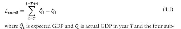
sequent years.
Expected output is calculated by applying a trend growth rate for output relative to working-age population to the annual growth in working-age population, with the base set as potential GDP in the year before the crisis. The use of working-age population is important because of the sharp demographic changes in the period after the Great Recession. Adjusting the base output level to the potential level addresses the problem of otherwise overstating the level of output that might have been expected by failing to recognize an unsustainable boom prior to the crisis.For its part, expected output is calculated as:

rate of growth of output per working-age population, and nt is the rate of growth of working-age population in year t. The multiplication operator ∏t refers to the cumulative product from period 1 to period t.
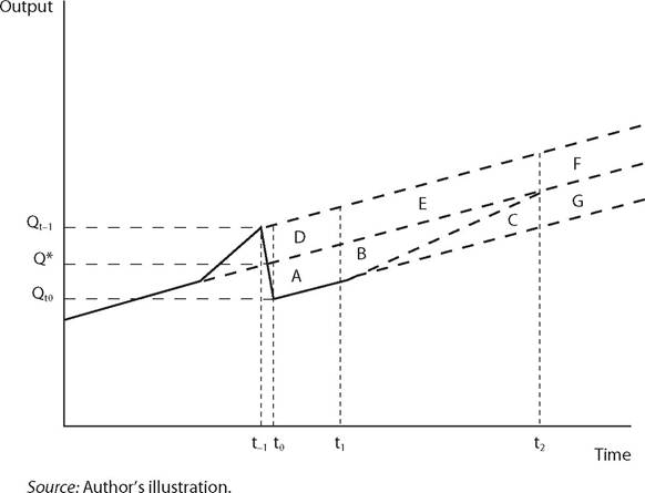
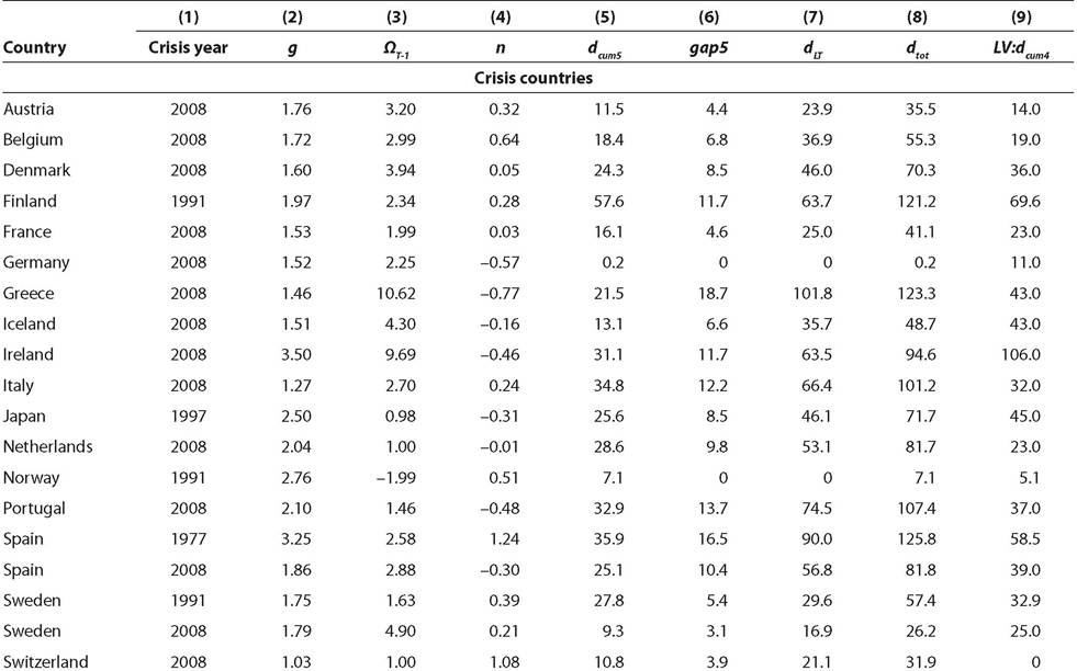
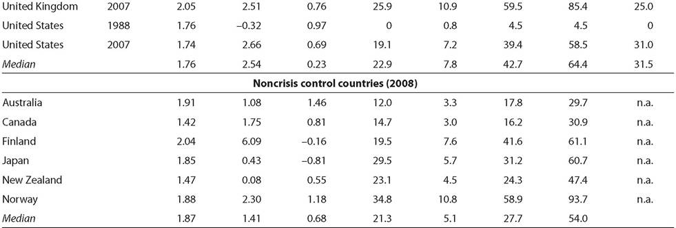
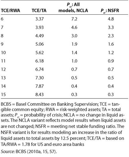
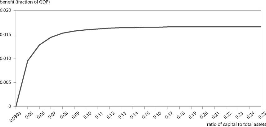
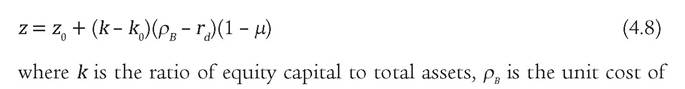
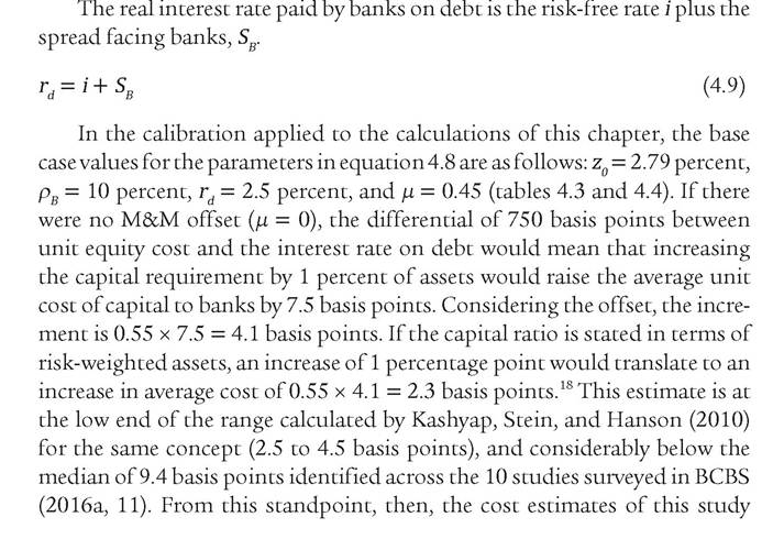
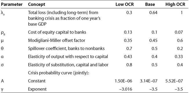
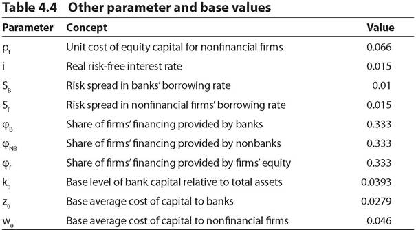
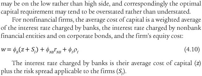
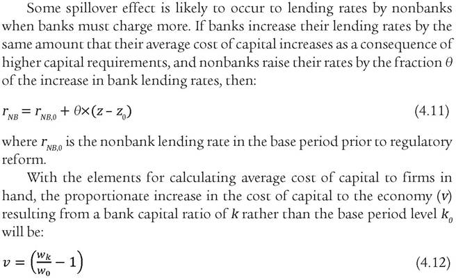
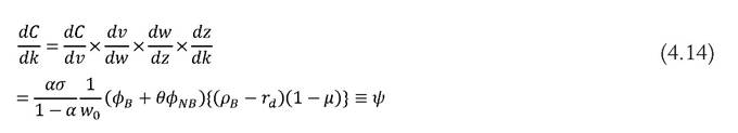
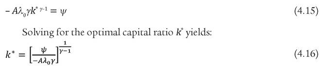
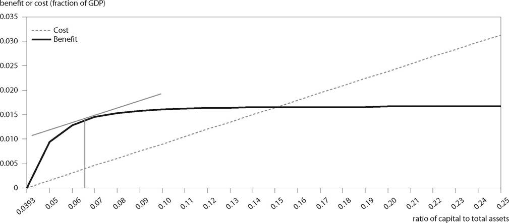
Long-Term Losses. In most of the banking crises, output does not fully return to its trendline by the end of the fifth year.[109] [110] A crucial question is then how to treat ongoing losses in later years. The approach here is to apply a finite lifespan of the “missing” capital stock and worker skills caused by the crisis, rather than interpreting the loss as persisting over an infinite horizon. In contrast, simply capitalizing the gap between output and trend still present in year 5 (or another year chosen as marking the end of the crisis) by dividing by the discount rate would implicitly assume that the extra capital equipment that would have been created during the crisis under normal circumstances would have had an infinite life. The approach here is to identify a lifetime M of the relevant productive capacity, and to apply straight-line depreciation. The present value of losses subsequent to Figure 4.1 Losses from a banking crisis Figure 4.1 illustrates the losses from a banking crisis. In an upper-bound estimate of output loss, there would be no reduc- 3. Note that the first five years involve no discounting, in part because with typically falling per capita income the usual intertemporal consumption basis for discounting (rising per capita consumption combined with diminishing marginal utility) is not present but also because the period is short enough for discounting to have limited influence. tion from the initial positive output gap, and losses would be assumed to last forever. In that case the loss would add not only areas C+G but also areas D+E+F (presumably with some time discounting to address the infinite horizon). Such an estimate, however, would be seriously exaggerated. Estimates of Losses from Banking Crises. By now a relatively standard set of episodes is recognized as banking crises (see BCBS 2010a, 39; Reinhart and Rogoff 2008; Laeven and Valencia 2012). For several decades after the Great Depression, banking crises were essentially absent in industrial countries. Even so, US and other industrial-country banks barely avoided a crisis from large exposure to Latin America in the region's sovereign debt crisis of the early 1980s, in part thanks to concerted lending and official sector support of adjustment programs (Cline 1984). Table 4.1 reports estimates for equations (4.1) through (4.3) for 22 banking crises in 1977-2008 in advanced industrial countries.[112] It also reports corresponding estimates for six advanced economies that escaped a banking crisis in the 2007-08 period. Column 1 indicates the year the crisis began. Column 2 reports the average growth rate of real GDP per working-age population from 1980 through 2014, for crisis episodes in 2007 or 2008. For earlier crises, the column shows the corresponding growth rate during the two decades prior to the crisis through year 5 after the crisis.[113] Table 4.1 Estimates of output losses from banking crises in advanced industrial countries, 1977-2015 id="Picutre 31" class="lazyload" data-src="/files/uch_group74/uch_pgroup295/uch_uch7168/image/image031.jpg"> Column 3 reports the International Monetary Fund's estimate of the output gap (in percent) in the year prior to the crisis (IMF 2015c).7 There is a positive output gap in all but two of the 22 episodes, suggesting the importance of adjusting the trend GDP estimates downward by the amount of the positive output gap (equation 4.2). Column 4 reports average annual growth in the size of the working-age population in the five years beginning the year of the crisis. This potential labor force shrank relatively rapidly in Germany, Greece, and Ireland after 2008; it also shrank in Portugal and Spain. The steepest decline, at about 0.8 percent per year, was in noncrisis Japan. Column 5 indicates the cumulative five-year loss of output against the benchmark potential GDP path, as a percent of potential GDP in the year before the crisis. The median five-year loss amounted to about 23 percent of base-year potential GDP. The final column of the table reports a similar estimate for four-year loss of output as calculated by Laeven and Valencia (2012). Those estimates are broadly similar, albeit somewhat larger—with a median of about 32 percent. The higher estimates reflect the absence of an adjustment for above-potential GDP in the base year in the Laeven-Valencia estimates, as well as their use of trend GDP growth (rather than actual working-age population growth). These differences make the estimates much more modest here for Ireland (31 percent, instead of 106 percent of GDP in the Laeven-Valencia estimates) and Greece (22 percent instead of 43 percent). There is also a sizable difference for the United States (19 percent of base GDP instead of 31 percent). Column 6 indicates the shortfall of output in year 5 from the benchmark baseline for potential GDP, expressed as a percent of the base-year potential GDP (in the year prior to the crisis). Column 7 indicates the longterm loss subsequent to year 5 (equation 4.3), as a percent of the base-year potential GDP.[114] [115] With a median of 43 percent of GDP, this cost is relatively large. Column 8 is the sum of the five-year cumulative loss and long-term cost, again as a percent of base-year potential GDP. The median total loss is 64 percent of GDP. The bottom panel of table 4.1 carries out the same calculations for what may be seen as a “control” group of advanced economies that did not experience banking crisis in the Great Recession. Three of these economies (Finland, Japan, and Norway) experienced banking crises in the 1990s but escaped the banking crises of 2007-08.[116] It turns out that the “losses” that would have been attributed for this period are also relatively high for these economies. The median five-year cumulative loss is about 21 percent of base-year potential GDP, surprisingly close to the 23 percent median for the crisis cases. The median total cost (including long-term) is about 54 percent of GDP, compared with 64 percent for the banking crisis cases. At the extreme, then, it could be posited that the contribution of the banking crisis to losses should be calculated as the excess of the estimates for the crisis group over the control group. If this approach were adopted, the marginal cost of the banking crisis, including the long-term cost, would be small—only 10 percent of base-year potential GDP even for the total cost including long-term. It might be argued that the losses in economies such as Canada and Japan were driven by external diseconomies of the banking crises in the United States and the euro area, and thus that the problem is underestimation of the banking crisis costs (rather than overestimation) for lack of including externalities. However, all of these control economies had some degree of excess demand as measured by the output gap in 2007, and it would have required dexterous macroeconomic management to avoid some degree of subsequent shortfall from potential output even in the absence of international spillover from economies with banking crises. Moreover, much of the loss of output in the euro area reflected a sovereign debt crisis, and with the exception of Ireland and to a considerably lesser extent Spain, this crisis did not stem primarily from banking crises (Cline 2014a, chapter 3). Essentially the worst global recession in 80 years imposed severe losses, and attributing the entirety of these losses to banking crises may overstate the cost of a typical banking crisis and thus the welfare gains from reducing the probability of such a crisis. Another complication is that the IMF's calculations of the output gap might be seen as endogenous to hindsight reflecting actual history rather than what might have been. For example, in October 2007 the IMF's estimate of the US output gap for 2007 was -0.5 percent of potential GDP, whereas in October 2015 its estimate of the 2007 output gap was +2.66 percent of potential GDP (IMF 2007b, 2015b). Similarly, whereas the median value of the initial output gap in table 4.1 is +2.5 percent, the corresponding median value for contemporary estimates by the IMF in 2008 (or, for the United States and United Kingdom, 2007) was -0.4 percent (IMF 2007a, 2008c). Yet it would seem inappropriate to completely ignore the benefit of hindsight. In the US economy, for example, the jeopardy that arose from the housing market bubble is now evident but was much less recognized in 2007. The analytical challenge is that an extremely wide range can arguably be asserted for the magnitude of banking crisis damages. As noted, the estimate could be as low as 10 percent of the base year's GDP, using the control group approach. At the opposite extreme, if it is assumed that there was no positive output gap before the crisis, and that the entire gap from the no-crisis baseline by year 5 should be seen as permanent, then the median damage from a banking crisis could be estimated as high as 450 percent of GDP![117] In the empirical estimates developed below, the central estimate of damage is placed at the 64 percent benchmark reported in table 4.1. The main calculations include alternatives at 30 percent and 100 percent of base-year GDP as what might be considered plausible-low and plausible- high estimates. However, in the discussion of the final results, the outcomes are also reported for two extremes: damage of 10 percent and 450 percent of base-year GDP. As will be shown, the resulting optimal ratio of capital to assets turns out to be considerably narrower than might have been thought for this 45-fold variation in the damage parameter. That outcome essentially reflects the sharp curvature of the function relating the probability of a banking crisis to the capital ratio, as developed below. Finally, it warrants mentioning that the damage estimates here are formulated in a binary nature: either zero, for no crisis, or a fixed estimate (64 percent of base-year GDP in the central estimate), if a banking crisis occurs. It would be useful to provide a graduated estimate of output loss that relates the depth of the loss, given a banking crisis, to the amount of bank capitalization. However, the few studies that attempt to link crisis severity to level of bank capitalization are insufficient to draw significant conclusions (BCBS 2010a, 17). Comparison with Basel Committee Estimates. In its 2010 survey of damages from banking crises, the Basel Committee on Banking Supervision (BCBS) assessed the long-term economic impact (LEI) at 19 percent of GDP with no permanent effects; 158 percent of GDP with permanent effects and an infinite horizon; and 63 percent for the “median cumulative effect across all studies,” which it also characterized as the case in which “crises have a long-lasting or small permanent effect on output” (BCBS 2010b, 10, 13). On the basis of the existing studies, the BCBS argued that a 1 percentage point reduction in the annual probability of a banking crisis would thus generate gross benefits of 0.19 percent, 0.63 percent, or 1.58 percent of GDP, depending on the degree of permanency of the losses.[118] It turns out that the estimates in table 4.1 are extremely close to the middle case of the BCBS. Namely, the median total loss of 64 percent of base GDP is almost the same as the survey median of 63 percent found by the BCBS for the middle (as opposed to high permanent) estimate, even though in contrast the present study is heavily dominated by actual experience from the 2007-08 crisis rather than for earlier periods (and includes a wider range of countries, including emerging-market economies). Similarly, the cumulative initial effect during the crisis years, 19 percent in the BCBS estimates, is fairly close to the median five-year cumulative effect estimated here (22.9 percent). The key difference in the damage estimates, then, is in the long-term “permanent” effects, as table 4.1 shows no estimates anywhere near 158 percent. The central reason again is the judgment that nothing lasts forever and that some form of productive resource lifespan must be taken into account in arriving at a meaningful “permanent” effect. There is another key contrast, however. It concerns the baseline frequency assumed for the incidence of banking crises. This incidence is crucial, because the product of the annual probability of a crisis and the damage cost of a crisis determines the expected damage from a banking crisis, and thus the amount of benefit that can be achieved by reducing the likelihood of a crisis. The BCBS (2010a, 39) places the annual probability of a banking crisis at 3.6 to 5.2 percent for “all BCBS countries” and 4.1 to 5.2 percent for G-10 countries. The slightly lower range for both concepts is from the compilation of crises by Laeven and Valencia (2008) and the higher range from Reinhart and Rogoff (2008). The frequency estimates are for the period 1985-2009.[119] It is by no means clear, however, why the starting point should be 1985. In table 4.1, there is a banking crisis recorded for Spain in 1977. If we begin the period at 1977 and bring it up to 2015, then there is a span of 38 years to consider. If we consider all the industrial countries listed in table 4.1 (including the “control” group with no crisis in 2008), there are 22 countries. The number of country-years in this full span is thus 836. The number of banking crises in table 4.1 is 22. On this basis, the annual frequency of a (new) banking crisis is 2.6 percent. At the upper end of the BCBS range for both frequency of and damage from banking crisis, the expected annual loss from a banking crisis under conditions of 1985-2009 was 5.2 percent ? 158 percent = 8.2 percent of one year's GDP. By this reckoning, if it were possible to purchase an insurance policy that would completely eliminate the risk of a banking crisis, it would be worth spending 8.2 percent of GDP every year to pay the premium on this policy. This amount would be several times what most countries pay for national defense. If instead the estimates of table 4.1 are adopted and the time span is set at 1977-2015, then the expected annual loss from banking crises amounts to 1.7 percent of GDP (2.6 percent ? 64 percent). Although still high, this estimate (which includes long-term effects) would seem more plausible than the 8.2 percent of GDP expected loss in the high end of the BCBS estimates. Even this lower figure could be exaggerated, however, to the extent that it mainly captures the extreme outcomes of the Great Recession, something broadly comparable to a 100-year flood that included losses from uncertainty associated with sovereign debt distress not necessarily triggered by banking crises. The Capital Requirements Benefits Curve. Let the probability of a banking crisis when the capital requirement is at its base level k0 be Pcr0. Let the total output loss from a banking crisis (including the long-term loss) be L. Defining the crisis loss as the fraction λ of one year's base GDP (Y0), where λ0 = Lcr /Y0, the annualized expected loss from a banking crisis expressed as a fraction of base year GDP will be: were from 2007 or 2008, constituting 54 percent of the G-10 banking crises in the period according to the first study and 78 percent according to the second. Calibrating the Benefits Curve. Arguably the most crucial and also the most uncertain building block in implementing the benefits model set forth in equations (4.4) through (4.7) is the curve describing the response of the probability of a banking crisis to the level of the bank capital requirement (equation 4.5). The most authoritative estimates on this question still seem to be those compiled in a survey by the BCBS in 2010 (BCBS 2010a). It is worth quoting from the study on its method: Mapping tighter capital and liquidity requirements into reductions in the probability of crises is particularly difficult. This study relies mainly on two types of methodology. The first involves reduced-form econometric studies. These estimate the historical link between the capital and liquidity ratios of banking systems and subsequent banking crises, controlling for the influence of other factors. The second involves treating the banking system as a portfolio of securities. Based on estimates of the volatility in the value of bank assets, of the probabilities and of correlations of default and on assumptions about the link between capital and default, it is then possible to derive the probability of a banking crisis for different levels of capital ratios. (BCBS 2010a, 3). Table 4.2 BCBS synthesis of impact of capital on the probability of systemic banking crises (percent) Key studies of the first type include Barrell et al. (2010) and Kato, Kobayashi, and Saita (2010). An example of the second category is Elsinger, Lehar, and Summer (2006). Table 4.2 shows the resulting synthesis of the BCBS mapping of capital ratios to banking crisis probability. The third and fourth columns of table 4.2 provide a basis for estimating the probability function in equation (4.5). If the logarithm of the crisis probability (column 3 or 4) is regressed on the logarithm of the ratio of capital to total assets (column 2), the resulting constant and coefficient estimates provide an estimate of A and g.[120] The point of departure for increasing capital ratios is a base of 7 percent tangible common equity relative to risk-weighted assets (3.9 percent of total assets), near the lower bound of the range considered in BCBS (2010a), as shown in table 4.2. At this level of capital, the probability of banking crisis is 4.6 percent in the all-models estimate and 3.3 percent in models considering liquidity and assuming that the net stable funding ratio (NSFR) liquidity targets are met. However, both these estimates are higher than the 2.6 percent benchmark identified above, based on 1977-2015 experience. As a result, in the main estimate here, the constant A is adjusted downward by the ratio 2.6/4.6.[121] Figure 4.2 shows the benefits curve relating the main estimate of losses avoided annually as a percent of total GDP in response to alternative ratios of capital to total assets. The zero point in these benefits is set at a starting point of 3.9 percent capital relative to total assets. The damages use the all-models estimates in table 4.2 (after the shrinkage from base crisis frequency of 4.6 to 2.6 percent). As can be seen, after the ratio of capital to total assets exceeds about 7 percent, the curve levels off, reaching a plateau of 1.67 percent of output. Thus, whereas the benefits of reducing the incidence of banking crises would amount to about 1 percent of GDP annually at a capital ratio of 5 percent, about 1.3 percent of GDP at a capital ratio of 6 percent, and about 1.5 percent at a capital ratio of 7 percent, boosting the capital ratio far higher to 25 percent would boost the benefits only marginally higher to 1.67 percent of GDP. This concave nonlinearity stems directly from the survey findings in BCBS (2010a). It is evident in figure 4.2 that the curvature of the benefits curve is quite pronounced in the range of capital to total assets of about 5 to 7 percent, but thereafter the curve is nearly flat. This phenomenon is a key driver of the optimal capital ratio estimates obtained below. The curvature of benefits is in turn driven by the curvature in the probability of banking crisis in response to alternative capital ratios (table 4.2). In explicating this crisis probability curvature, the Basel Committee report states the following: Another consistent result across models is that the incremental benefit of higher capital and liquidity requirements declines as the system becomes better capitalized. That is, when banks have low levels of capital, even small increases have a very significant impact, but the marginal benefit of further increases in capital ratios declines as banks move further away from the insolvency threshold.... These results are fairly intuitive. The Figure 4.2 Benefits of additional bank capital Source: Author's calculations. rationale is quite similar to that applying in the context of risk models applied to individual banks. For a given volatility in the value of assets, the further away a bank is from the insolvency threshold, the lower is the benefit of additional protection. (BCBS, 2010a, 16.) It is important to recognize that the 1.67 percent potential upperbound benefit refers to the level of GDP, not the annual growth rate. Thus, if extremely high capital requirements were set (say 20 to 25 percent of total assets), and there were no costs, the long-term path of GDP would be expected to lie about 1.7 percent higher than if there had been no change from the pre-Basel III requirements. The corresponding increase in the growth rate—again if there were no costs at all from higher requirements because of complete M&M offset—would amount to 0.055 percent annually over a 30-year period.[122] Costs of Higher Capital Requirements If the Modigliani-Miller offset is incomplete, however, higher capital requirements for banks will increase their costs. As they pass along these extra costs to borrowers, lending rates will rise. Firms borrowing capital will find it is no longer profitable to borrow as much and make plant and equipment investments as large as before. With less capital formation, total output will reach levels lower than otherwise. As will be shown, the output cost of higher capital requirements turns out to be a linear function of the level of the requirement, expressed as the ratio of equity capital to total (not risk- weighted) assets. Average Cost of Capital. The initial and driving force in the output cost is the increase in the interest rate banks must charge on loans as a consequence of shifting from cheaper debt finance to more expensive equity finance (under incomplete M&M effects). Thus, defining z as the average cost of capital to banks, one has: equity capital for banks, rd is the real interest rate on debt financing of the banks, and μ is an M&M offset factor.[123] Subscript 0 refers to the base period prior to the regime shift raising capital requirements. The analysis here refers to the ratio of equity capital to total assets, not risk-weighted assets. This ratio is sometimes called the “leverage ratio,” although it is actually a close transform of the inverse of the leverage ratio of debt to equity.[124] [125] Note further that regulatory requirements refer to capital required relative to “risk-weighted” assets. The values of risk-weighted assets (RWA) are considerably lower than those of unweighted assets because of the low risk weights for some assets (especially for highly rated sovereign obligations but also for home mortgages). In equation (4.8), if the capital ratio is increased from a modest base (say 5 percent) to a high level (say 25 percent), there will be a corresponding increase in the weighted-average cost of capital, reflecting the excess of the equity cost rate (pB ) over the borrowing rate facing the banks (rd ). The final term in the equation shrinks this increase in average cost of capital by the factor μ. If offset is complete (μ = 1), the average cost of capital to banks remains unchanged at z0 regardless of how high the capital requirement k is raised. Table 4.3 Alternative parameter values for simulations OCR = optimal capital ratio Source: Author's calculations. Source: Author's calculations. Impact on the Economy. As suggested by Miles, Yang, and Marcheggiano (2012) and followed in Cline (2015c), the proportionate output cost to the economy from placing the bank capital requirement at k rather than at the prereform level of k0 will then be: where α is the elasticity of output with respect to capital (capital's factor share) and σ is the elasticity of substitution between capital and labor. The derivative of this output cost with respect to the required capital ratio is then: and μ = 0.45. The resulting value of ψ, the constant derivative of output with respect to the capital ratio, is 0.15. Thus, for example, if the capital requirement is increased by 10 percent of total assets, the level of output will decline by 1.5 percent from the path it otherwise would have followed. Over 30 years, cumulative output loss would amount to 45 percent of the initial base-year output level, ignoring time discounting as well as the baseline growth rate.[126] This illustration makes it evident that the economic cost of a large increase in capital requirements would be substantial. Identifying the optimal level of capital thus requires a close examination of the marginal cost in comparison to the marginal benefit. The estimate for ψ developed here is extremely close to that identified for the corresponding concept in the LEI study (BCBS 2010a, 26). That study found that across 13 models, the median impact of an increase by 1 percentage point in capital relative to risk-weighted assets was a reduction of 0.09 percent in the level of production. With risk-weighted assets only 56 percent of total assets, the corresponding impact of an increase in capital by 1 percent of total assets would amount to an output reduction of 0.16 percent, almost the same as the parameter ψ = 0.15 estimated in the present study. Because the LEI analysis conservatively sets the M&M offset at zero, it follows from equation (4.14) that the BCBS parameter for ψ should be more than twice as large as the magnitude in the analysis here.[127] By implication, the LEI study seems to understate the long-term output cost resulting from a specific realized increase in the unit cost of capital to firms. Two sources of that underestimation seem likely. First, the studies surveyed in the LEI study may tend to use a higher base unit cost of capital than the level applied here (4.6 percent in real terms; see table 4.3). If so, a specific increment in the unit cost of capital in the LEI study would be a smaller proportionate increase than in the calculations here. Second, the LEI survey includes simulation results from large macroeconomic models. These models may understate output effects by inappropriately including monetary policy offsets reducing the policy interest rate, even though an environment of less capital stock formation would imply greater scarcity and if anything more severe inflationary pressures. Moreover, these models seem more likely to be relevant for evaluating consequences of shifts in demand than long-term shifts in capacity and underlying supply. Optimal Capital Requirements With the marginal social cost of additional capital given by equation (4.14) and the marginal social benefit given by equation (4.7), the optimal capital ratio k' will occur where these two marginal effects are equal, at: In graphical terms, this optimal capital ratio will occur where the slope of the convex benefit function equals the slope of the linear cost function. Tables 4.3 and 4.4 report parameter values applied in implementation of the model using equations (4.4) to (4.16). For seven key influences shown in table 4.3, three alternative parameter values are considered: a base case using the central estimates; a “low” case in which the parameters will generate a lower optimal capital ratio (with other parameters unchanged); and a “high” case in which the parameters will generate a higher optimal capital ratio (OCR). The first parameter, λg, is the expected present value of damage from a banking crisis, as a fraction of one year's base GDP. The estimates in table 4.1 provide the central value of 0.64 for this parameter. The low OCR variant is set at 0.30 (effectively treating most of the damages as those occurring within the first five years); the high OCR variant, at 1.0, represents much longer persistence of damages. For the second parameter, pB, the unit cost of equity capital, the base case uses 10 percent. This is the rate indicated in IIF (2011). For the two alternative rates, 13 percent and 7 percent, the source is chapter 3, table 3.1. These were the rates identified for 54 large US banks in 2001-13 for the earnings yield (inverse of price-to-earnings ratio) and the ratio of net income to equity, respectively. The 13 percent equity cost variant will impose greater costs from forcing a shift away from debt to equity, so it represents a low-OCR case; conversely, a 7 percent equity cost represents a high-OCR case. The base case places the M&M offset, μ, at 0.45, again based on the estimates in chapter 3. The low-OCR alternative posits a smaller offset of 0.35; the high-OCR alternative sets the offset at 0.6. For the spillover effect, θ, the base estimate assumes that nonbank lending rates rise by one-half of the increase in bank lending rates. The low-OCR variant sets this spillover effect at 0.7, raising the economic cost of higher capital requirements for banks; the high-OCR variant assumes a spillover coefficient of only 0.2, making higher capital requirements less costly. The base elasticity of output with respect to capital, α, is set at 0.4, reflecting the high share of capital in GDP in recent years. As can be seen in equation (4.13), the economic cost of higher capital requirements is positively associated with α. Higher cost translates to a lower optimal capital ratio. The low-OCR variant of α is set at 0.43. Conversely, the high-OCR variant is set at the more traditional notional value of α = 0.33.[128] The elasticity of substitution, σ, is set at 0.5 in the base case (following Miles, Yang, and Marcheggiano 2012). Again equation (4.13) reveals the direction of influence of this parameter on economic cost of higher capital requirements as being positive. The low-OCR variant is thus set at 0.8 (higher cost will lead to a lower optimal capital ratio), and the high-OCR variant, at 0.4.[129] The final two rows of table 4.3 show alternative sets of parameters for the crisis probability curve. The base case applies the “all models” column of table 4.2, but imposes the base crisis probability estimate of 2.6 percent developed in the initial section above. The high-OCR alternative instead accepts the BCBS (2010a) base crisis probability of 4.6 percent and applies the curvature of the all-models estimates (table 4.2). That is, with higher crisis damages and hence benefits of curbing the probability of crisis, there will be a higher return to additional bank capital. The low-OCR variant imposes the lower 2.6 percent base probability of crisis, and applies the somewhat more favorable curvature of the net stable funding ratio estimates in the BCBS (2010a) study. For the other parameters and base values in the model, single estimates are applied, as shown in table 4.4. Equity cost to firms is based on a typical price-to-earnings ratio of 15.[130] A real risk-free interest rate of 1.5 percent is meant to represent medium- to long-term rates under conditions more normal than those following the Great Recession. The risk spread for banks is based on observed credit default swap rates.[131] The share of equity in corporate financing is set at one- third on the basis of data for G-7 countries (Rajan and Zingales 1995, 1428). The share of debt financing by corporations is also set at one-third as estimated by Miles, Yang, and Marcheggiano (2012, 16), who note that this share would be lower for the United States and “slightly higher” in some European countries. The remaining share of capital financing, in the form of nonbank debt (including corporate bonds) is then also one-third. The base value of the capital-to-assets ratio is set at 3.93 percent, based on the base value of 7 percent for tangible common equity relative to risk- weighted assets and a ratio of 1.78 for total assets to risk-weighted assets for US and euro area banks (BCBS 2010a, 57). The two final entries in table 4.4 are the estimated base values of average cost of capital to banks and average cost of capital to nonfinancial firms, obtained by applying equations (4.8) and (4.10) to the parameters and base values in tables 4.3 and 4.4. Results Application of the base case values for the parameters in tables 4.3 and 4.4 yields an optimal capital-to-assets ratio of k' = 0.0656. Figure 4.3 shows the paths of benefits (equation 4.6) and costs (equation 4.13), using the base case. As noted, in this case the total potential benefit of higher capital ratios plateaus at about 1.7 percent of annual GDP. If the capital-to-assets ratio were raised all the way to 25 percent, the cost would reach 3 percent of annual GDP. The two curves intersect at a capital-to-assets ratio of about 15 percent. But the optimal capital ratio, the point at which the slopes of the two curves are parallel, occurs at a capital-to-assets ratio less than half as high, at 6.56 percent. This optimal ratio would correspond to a ratio of capital to risk-weighted assets of 11.7 percent. Figure 4.4 provides a histogram of the estimates of the optimal cap- ital-to-assets ratio across all 2,187 possible combinations of parameters in table 4.3 (again calculated using equation 4.16). The lowest optimal ratio is 0.0411. The highest estimate finds k* = 0.1164. At about 12 percent, even the highest case is slightly less than half of the midpoint of the 20 to 30 percent range recommended by Admati and Hellwig (2013, 179). The median estimate of the optimal capital ratio is k* = 0.0694 percent, slightly higher than the base case estimate (k* = 0.0656). When arrayed from lowest to highest, the 25 th percentile shows a value of k* = 0.0611, and the 75th percentile places k* at 0.0787. On this basis, it seems reasonable to place the central estimate of the optimal capital ratio at about 7 percent of total assets, and a more risk-averse main estimate at about 8 percent. Returning to the issue of potentially wide variation in the estimated damage from a banking crisis, it is useful to consider the optimal capital ratios implied by the extreme ends of the spectrum discussed above. If a banking crisis causes output loss of only 10 percent of base-year GDP (λ0 = 0.1), and if all other parameters in tables 4.3 and 4.4 are set at their base values, then the optimum capital ratio reaches only 4.3 percent of total assets (k* = 0.043). If instead banking crisis damage is set at 450 percent of Figure 4.3 Benefits and costs of additional bank capital Source: Author's calculations. Figure 4.4 Frequency of estimates for optimal capital-to-assets ratio Source: Author's calculations. GDP (λ0 = 4.5), the optimal capital ratio rises to 10.1 percent of total assets (k' = 0.101), higher than the 75th percentile in the main estimates but lower than the very highest estimate (11.6 percent) identified from the most extreme combination among the alternative parameters already considered. An important question is whether the optimal range identified here should be substantially different for European as opposed to US banks, in view of the greater reliance on bank finance in Europe. This question can be examined by changing the shares of debt finance to the economy between banks (φB ) and nonbanks (Φnb ). The consequence of a higher bank share will be to raise the economic cost of higher capital requirements for banks. Merler and Veron (2015, 54) estimate that whereas 88 percent of corporate borrowing in the euro area comes from banks, this share is only 30 percent in the United States. Applying these shares to the combined two-thirds of finance coming from debt, the parameter φB would be placed at 0.59 for the euro area but only 0.2 for the United States (leaving the parameter Φnb at 0.08 or 0.47, respectively). From equation (4.14), the effect of applying these tailored financing shares is to change the cost parameter ψ from 0.15 percent of GDP for each percentage point increase in the capital-to-total assets ratio, to 0.19 percent for the euro area and 0.13 for the United States. Equation (4.16) can then be applied to obtain the corresponding changes in optimal capital ratios. With k* as the optimal capital requirement in the base case, the tailored debt-sourcing shares place the optimal capital ratios at kε' = 0.965 k* for the euro area and ku' = 1.022 k* for the United States.[132] So even a seemingly high divergence between bank and nonbank sourcing of debt has only a modest impact on the optimal capital ratio. Namely, the US optimal ratio would be proportionally higher than the euro area optimal ratio by only about 6 percent, even though the unit economic cost of capital would be 46 percent higher (ψ = 0.19 versus 0.13). This exercise once again underscores the importance of the high degree of curvature in the benefits curve, which is based on the BCBS (2010a) estimates of the sharp drop-off in crisis probability as the capital ratio increases (table 4.2). This same influence is the driving force behind the relatively modest change in the optimal capital ratio (from 4.3 to 10.1 percent of total assets) as crisis damage is multiplied 45-fold between the extreme variants just noted. Because of this key influence, further research is warranted on whether the BCBS estimates provide the right degree of curvature in the relationship of crisis probability to the capital ratio.[133] Comparison with Other Estimates Alternative estimates in four other studies warrant special discussion. The first two are important in their own right but also provide key inputs for the estimates here. The third is a benchmark academic study, and the fourth a recent empirical study conducted at the IMF. First, in its summary assessment, the 2010 Basel Committee study that provides the basis for the crisis probability estimates here identified an optimal ratio of capital to risk-weighted assets (TCE/RWA) of 10 percent if there are no permanent effects of banking crises, and 12.5 percent if there are “moderate” permanent effects (BCBS 2010a, 2). The moderate permanent effects case is close to the 11.7 percent identified here (6.56 percent of total assets). There is, nonetheless, an important difference. As shown in figure 4.3, net benefits—the vertical distance between the benefits curve and the cost line—show a steady and sizable decline after capital exceeds the optimal ratio. In contrast, in the BCBS study the net benefits remain almost flat at about 1.7 percent of GDP even as the ratio of capital to risk- weighted assets reaches 16 percent. This level corresponds to a ratio of about 9 percent for capital relative to total assets. At this level, net benefits (the distance between the upward-sloping line for cost and the convex curve for benefits) would be significantly smaller than at the optimal ratio.[134] The reason for the seeming flatness of the net benefits curve in the BCBS study is not clear. This pattern appears to reflect a nonlinear cost curve that allows for costs to plateau almost as fully as benefits. The study's cost estimates are opaque, however, as they are based mainly on several dynamic stochastic general equilibrium (DSGE) models without details reported. Second, Miles, Yang, and Marcheggiano (2012) use a framework similar to that applied here. Although specific components and calibrations differ, their overall results are similar to those obtained here. On the side of economic costs of additional capital, their cost curve is only about half as steep as that developed here, largely because they set their base value for the average cost of capital to firms at about twice the level assumed here.[135] Their benefits curve is quite different in concept, and is premised on the proposition that a given decline in GDP causes an equal and proportionate decline in risk-weighted assets. The distribution of asset reductions is then compared with capital to estimate the implied incidence of banking crises. They obtain a distribution of GDP declines based on 200 years' data for 31 countries. The authors set the present value of a banking crisis at a loss of 55 percent of one year's GDP—a benchmark similar to the 64 percent base estimate here. If they exclude the most extreme cases (where GDP falls by 35 percent), it turns out that their optimal capital ratio lies in the range of 7 to 9 percent of total assets.[136] That range is surprisingly close to the range identified here: 6.56 percent of total assets (base case) to 7.9 percent (conservative 75th percentile). The third and fourth studies warranting special mention are those by Admati and Hellwig (2013) and Dagher et al. (2016). Both are reviewed in chapter 2. The Admati-Hellwig recommendation of bank equity capital of 20 to 30 percent of total assets is far above the range found optimal here. It is not based on an optimization model. The recent IMF study by Dagher et al. (2016), in contrast, arrives at a desired range for capital that is comparable to that estimated in this chapter. Finally, the “Minneapolis Plan,” issued in preliminary form by the Minneapolis Federal Reserve in late 2016, uses the Dagher et al. (2016) data on the relationship of crises to nonperforming loans and bank capital, together with simulations of the Federal Reserve's large macroeconomic model to arrive at an optimal capital ratio of 23.5 percent of risk-weighted assets. For the reasons set forth in appendix 4A, this estimate appears to be seriously overstated. Implications for Regulatory Capital The Basel III regulatory reform requires that by 2019 banks hold a minimum of 4.5 percent of risk-weighted assets in common equity, plus another 2.5 percent as a capital buffer (BCBS 2010b, 69). The total requirement of 7 percent of RWA in common equity corresponds to 3.9 percent of total assets.[137] G-SIBs are to hold additional capital of up to 2.5 percent of RWA, bringing the ratio to 9.5 percent of RWA (BCBS 2014c).[138] A capital ratio of 9.5 percent against risk-weighted assets corresponds to a ratio of 5.3 percent against total assets. Against the optimal ratio estimated here—6.6 percent central estimate and 7.9 percent for the conservative 75th percentile estimate—the Basel III capital requirements are too low. They would need to rise by about one-fourth to reach the central estimate, and by about one-half to reach the more risk-averse 75th percentile estimate. Even so, the increases needed to reach the optimal capital ratios are far less than the five-fold multiple called for by Admati and Hellwig (2013). In the United States, the additional amount for G-SIBs is to range up to 4.5 percent, bringing the ratio to as high as 11.5 percent of RWA.[139] This level would correspond to 6.5 percent of total assets. That level would be almost exactly the same as the base case optimal capital ratio identified in the present study. However, in practice the highest G-SIB increment by early 2016 was 3.5 percent (for JPMorgan), and the amount for the US G-SIBs was centered at about 3 percent.[140] So the principal G-SIB rate stood at about 10 percent of RWA, or 5.6 percent of total assets. On this basis, even for US G-SIBs the capital requirement would need to increase by about one-sixth to reach the central-estimate optimal capital ratio and by about two-fifths to reach the more conservative benchmark (6.56 and 7.9 percent, respectively). The G-SIBs account for a large portion of assets in the international banking system. The broad implication is thus that capital requirements on track under Basel III are below optimal levels, but not nearly as far below as some past studies have suggested. Table 4.5 Basel III and FSB capital requirements for G-SIBs FSB = Financial Stability Board; G-SIBs = global systemically important banks; TLAC = total loss-absorbing capacity a. Includes goodwill, deferred tax assets, some contingent convertible debt. b. Other contingent convertible debt, subordinated debt. Sources: BCBS (2010b, 2014c); FSB (2015d). Table 4.5 summarizes Basel III requirements for G-SIBs, and in addition reports the TLAC requirements recommended by the Financial Stability Board in response to the St. Petersburg Summit of the Group of Twenty (G-20) in 2013 (FSB 2015d). The Basel III requirements are to be met by 2019; the TLAC target is to be met by 2022. The table shows the requirements in the usual form, against risk-weighted assets, and also the corresponding central estimate of the implied ratios against total assets.[141] Because the TLAC target is to be assessed on an individual bank basis, the 18 percent shown in the table is a minimum for G-SIBs.[142] The analysis in this study is based on the tangible common equity concept of capital. This metric is used to calibrate the relationship between the probability of banking crisis and the level of capital (table 4.2). The proper comparison thus contrasts a Basel III target of 9.5 percent of RWA against an optimal range of about 12 to 14 percent identified in the present study. As shown in table 4.5, however, the further requirement for TLAC pursued by the G-20 and Financial Stability Board would bring TLAC up to 18 percent of RWA. A key question is thus whether this additional layer would constitute an effective achievement of the optimal 12 to 14 percent range. Chapter 5 examines contingent convertible (CoCo) debt and subordinated debt that would constitute the increment that would approximately double TCE to reach the TLAC level. The discussion there suggests that TLAC does not adequately address the basic purpose of capital, which is to ensure that the bank remains solvent. Instead, it is designed to ensure that a large bank can indeed go bankrupt without requiring a call on taxpayer funds. Subordinated debt could be subtracted from the bank's debt liabilities only upon bankruptcy. Bankruptcy of large banks is precisely what capital requirements should be designed to avoid, considering that episodes of failure of large banks would be difficult to envision without an associated banking crisis. As for CoCo debt, in a panic the collapse of market values of this debt would hardly contribute to an atmosphere favorable to avoiding broader crisis (Persaud 2014).36 Moreover, US banks have not used CoCo debt because its interest does not qualify as a tax-deductible expense. Further Considerations Three major additional issues warrant reflection in interpreting the results of the estimates here. The first is whether consideration of social versus private returns substantially alters the diagnosis. The second concerns the relationship between capital actually held by banks and the amount required by financial regulations. The third concerns the possibility that decisions in monetary policy could change the regulatory policy calculus. Social versus Private Returns. Admati et al. (2011, 22-23) argue that even if higher bank capital requirements cause an increase in bank lending rates, the result is likely to be welfare-enhancing from the viewpoint of society as opposed to private shareholders and borrowers. Their reason is that existing government guarantees of deposit, as well as implicit guarantees of too big to-fail, give a distorted incentive to banks to take excessive risks that can damage the economy in a financial crisis. These distorted incentives are additive to the general distortion from tax favoritism to debt relative to equity. Identifying socially optimal increases in bank capital, however, would require taking into account a realistic evaluation of costs to the economy from raising bank lending rates and as a consequence reducing capital for- [143] mation. It may well be that the corresponding reduction in expected social losses from financial crises would warrant substantial costs from lower capital formation. But in principle there is likely to be some optimal limit to the socially beneficial increase in capital if the operational effect is some loss in output because the M&M offset is in fact far from complete. It is further worth noting that social benefits are associated with the service of providing bank deposits, because they constitute money performing its three basic functions: liquidity, store of value, and medium of exchange. It is not clear that the social subsidy to banks from government deposit guarantee is greatly larger than the social externality provided by banks in the form of providing money in the form of deposits. In short, although recognition of the need to take societal externalities into account could indeed lead to identification of optimal capital requirements that are significantly higher than in the past, the calibration of appropriate policy is considerably more complicated than implied by a general proposition that higher capital requirements are costless and existing capital arrangements subsidize banks and encourage them to take risks at the expense of the public. Behavioral Cushions. In practice, in the United States (at least) the large banks have already reached capital ratios that not only exceed the Basel III requirements but also are close to the optimal levels identified in this study. In the fourth quarter of 2014, 31 large bank holding companies (representing more than 80 percent of total bank assets) held Tier 1 common equity amounting to 11.9 percent of risk-weighted assets (Federal Reserve 2015c, 3). The Basel III requirement, including the G-SIB surcharge as applied in the United States (an average of 3 percent), is 10 percent of RWA.[144] So these banks held one-fifth more capital than the regulatory requirement (and well before the 2019 deadline). For these large banks, the ratio of total assets to RWA was an average of 1.53 (ibid.). So their common equity was 7.8 percent of total assets—effectively at the conservative (75th percentile) side of the optimal level estimated here. The question thus arises as to whether the Basel regulatory requirement should be raised to the optimal level or instead placed significantly below the optimal level because of the banking practice of maintaining a cushion. As a principle of public policy, it would seem unwise to count on voluntary overachievement of regulatory requirements. The proper approach would be to set the capital requirement at the socially optimal level, and to anticipate that at the newly higher level banks would no longer maintain such large cushions of additional capital beyond the required amounts. In the estimates above, the central result for optimal capital is 6.6 percent of total assets. If banks maintained a cushion of an additional one- fifth, their capital would stand at 7.9 percent of total assets. As it turns out, this is the same as the conservative alternative (75th percentile) estimated here for the optimal ratio. The reasonable policy approach, then, would seem to be to set the regulatory requirement at the central estimate of the optimal level, in the expectation that in practice the banks would add a cushion that places their actual capital levels at the conservative (75th percentile) optimal target. Monetary Policy Offset? Another key consideration is whether the costs of additional capital could easily be offset by more expansionary monetary policy, essentially achieving greater bank capitalization at no cost to the economy. The problem with this line of thinking is that monetary policy should stick to its central mandate—maintaining price stability along with high employment—and not be burdened with extraneous obligations. Superficially the numbers do look congenial to the monetary offset argument. Specifically, increasing the capital requirement by as much as 10 percent of total assets would raise the cost of capital to the economy by “only” about 20 basis points.[145] This amount is substantial relative to the average cost of capital to the economy (4.6 percent in the base case, with the increment representing a proportionate increase of 4.3 percent in the unit cost of capital). However, it would be equivalent to only a modest loosening of monetary policy (e.g., reducing the policy interest rate from 3 to 2.8 percent, or by 20 basis points).[146] But an environment of reduced capital formation and consequently lower output would tend to be one of supply scarcity rather than demand deficiency. Supply scarcity would tend to boost inflationary pressures, so that if anything a monetary policy response could be more likely a tightening than a loosening. Essentially, long-term financial regulatory structure should not be premised on the pursuit of monetary policy more expansionary than otherwise advisable. Conclusion This chapter finds that long-term damage of a banking crisis amounts to 64 percent of base-year potential GDP and that in the past three decades the annual probability of such a crisis was about 2½ percent. The probability of a banking crisis can be reduced by requiring banks to hold more capital. The response of crisis probability is highly nonlinear, such that the most impact in reducing chances of a crisis comes from the initial increases in capital above pre-Basel III levels. After taking account of the additional cost to the economy from imposing higher capital requirements (thereby raising lending rates and curbing new investment and future output levels), it is found that the optimal ratio for tangible common equity is about 6.6 percent of total assets and a conservative estimate at the 75th percentile is about 7.9 percent. These benchmarks would correspond to 11.7 and 14.1 percent of risk-weighted assets, respectively. On this basis, the Basel III benchmarks are below optimal capital requirements, at only 7 percent of RWA (9.5 percent for G-SIBs). Further international banking reform could usefully consider phasing in capital requirements on the order of one- fourth to one-half higher than the Basel III requirements. Appendix 4A An Evaluation of the Minneapolis Plan to End Too Big to Fail In late 2016 the Federal Reserve Bank of Minneapolis issued a Plan to End Too Big to Fail (Minneapolis Plan 2016).[147] The Minneapolis Plan (MP) study finds that the optimal level of capital for banks is 23.5 percent of risk- weighted assets. This level is nearly twice as high as the optimal level identified in the present study, a range of 12 to 14 percent. As a separate policy issue, the report goes on to argue that global systemically important banks (G-SIBs) should face a capital requirement of 38 percent, providing a strong incentive for these banks to split into smaller entities. The 38 percent level is chosen on grounds that it is at this level that the cumulative costs to the economy of higher bank capital requirements would begin to exceed the cumulative benefits from reduced risk of banking crises. The marginal costs would exceed the marginal benefits already at the lower optimal level, 23.5 percent. This appendix replicates the MP method and findings and seeks to clarify why its results are so different from mine. The discussion closes with additional observations about the too big to fail (TBTF) surcharge. Replicating the Minneapolis Plan Results The Minneapolis Plan (2016, 31) uses the Dagher, Dell'Ariccia, Laeven, Ratnovski, and Tong (2016, 13), or DDLRT, compilation of data on nonperforming loans in 28 banking crises in 24 OECD countries over the period 1970-2011 as the basis for mapping the probability of crisis to the amount of bank capital. The MP authors reason that there is a base crisis risk that equals 28 episodes divided by 42?24 country years, resulting in a probability of 2.78 percent in any given year that a country will have a crisis. They accept the DDLRT proposition that in each case the crisis would not have happened if banks had held capital equal to losses. They impute losses at either 50 percent of reported nonperforming loans (NPLs) or 75 percent of NPLs. DDLRT compare these imputed losses to total bank assets, which are typically about twice the loan book. After taking account of the fact that risk-weighted assets (RWA) are typically only about 57 percent of total assets, DDLRT are then able to identify the ratio of capital to RWA that would have been needed to cover the losses and avoid the crisis. DDLRT present a figure with the probability of avoiding a crisis mapped against the ratio of capital to risk-weighted assets, k. The MP authors use this mapping to calculate the probability of a crisis. I have estimated the following equation using the DDLRT figure and setting the value of k halfway between the 50 and 75 percent loss given default (LGD) lines shown separately in their figure (with t-statistics in parentheses): and k is the ratio of capital to risk-weighted assets (percent). Figure 4A.1 shows the cumulative probability of avoiding a banking crisis as a function of the ratio of capital to risk-weighted assets, and displays the corresponding estimated curve. The MP authors use the same DDLRT dataset and also use the midpoint of the 50 to 75 percent LGD alternatives. They then translate these probabilities into benefits from higher capital in the following way. First, they set the damage from a crisis at 158 percent of one year's GDP. This high level is meant to emphasize permanent losses; in contrast, I estimate the loss at 64 percent of one year's GDP after recognizing that the base year output is typically above potential and (more importantly) that “permanent” losses are not eternal because the capital assets that would have been built in the absence of a crisis would not have had infinite life (table 4.3). So in short, the MP authors apply crisis damage that is 2.47 times the size of the corresponding damage in the present study. Second, the MP authors identify the actual probability of a crisis as being equal to the base average of 2.78 percent, minus the influence of the reductions in the probability at successively higher levels of capital. Namely: However, this formulation would seem to involve a logical ellipsis. The procedure implicitly assumes that the observed average incidence of crises (2.78 percent) would have been no higher if there had been zero capital, but surely that is not the case. A major problem with the MP study is thus that it understates the probability of crisis at the lower end of the capital ratio spectrum. Third, the benefit to the economy from any given level of capital is then calculated as the base expected loss from crises multiplied by the probability of avoiding a crisis. With the crisis loss set at 158 percent of GDP and a base crisis probability of 2.78 percent annually, the expected crisis cost annually is 4.4 percent of GDP. The benefit of bank capital in the MP study is thus: Figure 4A.1 Probability of avoiding a banking crisis as a function of capital/risk-weighted assets These calculations thus successfully replicate the MP result for the optimal capital ratio when that study's parameters are applied for benefits of crisis avoidance achieved and cost to the economy of additional bank capital. Problems with the Estimates of Benefits There are two problems, in my view, with the MP estimates of crisis avoidance benefits as a function of bank capital. First, as noted, they implicitly assume that if bank capital were zero, there would be no more crises than had actually been observed in the reference period. Second, they assume a level of damage (158 percent of one year's GDP) that is implausibly high after taking account of the finite life of any capital assets that failed to be built during the crisis-induced recession. Figure 4A.2 compares the MP crisis probability curve to that presented in BCBS (2010a). The BCBS analysis is based on models developed by the UK's Financial Services Authority, Bank for International Settlements, and the central banks of Canada, Japan, and the United Kingdom. The estimates are based on econometric studies of historical experience relating crises to the amount of bank capital, as well as models of the banking system as a portfolio of securities. The models show a relatively rapid drop-off in the probability of a crisis as the capital/RWA ratio rises, a phenomenon familiar from risk models applied to individual banks (BCBS 2010a, 16). Although the BCBS study remains the most authoritative evaluation of the relationship of crisis probability to bank capitalization, the MP authors prefer the DDLRT approach because it is “easier for an outsider to re-create and judge” and because “the direction of the worldwide regulatory community” more recently has been toward higher capital than implied by the BCBS estimates (Minneapolis Plan 2016, 20).[148] As shown in figure 4A.2, the MP crisis probability starts out far lower than that of the BCBS, and follows an extremely flat path such that after bank capital exceeds about 10 percent of RWA the MP crisis probability exceeds that in BCBS (2010a). The extreme flatness of the MP crisis probability curve means it is highly likely that the point at which its slope equals that of the economic cost curve will be at a much higher capital ratio than in the BCBS curve. As can be seen in figure 4A.2, the two alternative crisis probability curves are still not quite parallel (i.e., still do not have identical slopes) even at the top end of capital considered by the BCBS (15 percent of RWA). Figure 4A.2 Probability of a banking crisis as a function of bank capital/risk-weighted assets, Basel Committee on Banking Supervision versus Minneapolis Plan Sources: BCBS (2010a, 15); Dagher et al. (2016, 15); Minneapolis Plan (2016); and author's calculations. One reason for the flat MP curve is that the top four observations among the 28 OECD cases involve crises with exceptionally high losses, namely Iceland (2008) with peak NPLs at 60 percent of loans, and Japan and Korea (both 1997) and Greece (2008) at peak NPLs of about 35 percent of loans. In contrast, the median peak NPLs for the OECD crisis cases were only 10 percent of loan value (Dagher et al. 2016, 13). It would seem questionable whether it is socially cost effective to base US capital requirements in part on such extreme experiences.[149] Understatement of the Cost Curve Unlike Admati and Hellwig (2013), the MP authors do not obtain a low cost of capital requirements by assuming a complete “Modigliani-Miller offset” whereby shifting from low-cost debt to high-cost equity does not raise the average cost of capital because equity markets reduce the unit cost of equity in response to the resulting reduction in risk. They apply an offset parameter of one-half, about the same as the 0.45 magnitude estimated in chapter 3. Instead, the low cost in MP appears to stem from the use of the large macroeconomic model of the US Federal Reserve to calculate the impact of higher bank capital cost on GDP. The authors apply the Taylor rule to allow monetary policy to respond to a shock in the loan rate. But the Taylor rule is designed to address relatively short-term cyclical issues for which the concern would be excess capacity. Instead, the long-term economic cost of higher capital cost involves less underlying capital stock and productive capacity, such that if anything the relevance of the Taylor curve would be that it would recommend raising the policy interest rate rather than reducing it given incipient inflationary pressure from supply constraints. It is misleading to assume that there is a monetary policy offset that can substantially reduce the cost of lesser supply as a consequence of higher capital requirements. Nor is it clear that the Fed model is appropriate for long-term analysis more generally.[150] [151] The resulting cost parameter in MP is that an increase in the capital requirement by one percentage point of RWA causes a reduction of the longterm output path by 0.058 percentage point. The corresponding parameter in this study is 0.084.46 My estimate is based on the much more transparent approach proposed by Miles, Yang, and Marcheggiano (2012), which uses a simple aggregate production function. The higher unit cost of capital reduces capital formation and output declines in response to the factor share of capital and the elasticity of substitution between capital and labor. A simple test of the plausibility of the MP cost parameter is to consider the output impact of a specified capital cost increase. In their “step 2” G-SIB exercise, the MP authors set the capital requirement at 38 percent of RWA. They calculate that this level would boost loan rates by 1.43 percentage points above those under current regulatory requirements. The same increase would apply to nonbank financial intermediaries in the MP (to avoid regulatory arbitrage). If we assume that banks and nonbanks together supply two-thirds of finance to nonfinancial corporations and the rest comes from retained earnings and new equity issuance, the economywide cost of capital would rise by 0.96 percentage point. I place the average real unit cost of capital to nonfinancial firms at 4.6 percent (table 4.4). So an increase of 96 basis points would amount to a 21 percent proportionate increase in the cost of capital to the economy. In the simple aggregate production function approach, a proportionate increase of z in the unit cost of capital causes a reduction of z ? [ασ]∕[1-α], where α is the share of capital in output and σ is the elasticity of substitution between capital and labor. In the example here, with z = 21 percent, a capital share of 40 percent (α = 0.4) and an elasticity of substitution of σ = 0.5, the impact would be a reduction of output by 7 percent. Yet the MP estimate for the step 2 impact is a reduction of output by only 1.41 percent (Minneapolis Plan 2016, 22). The mechanics of the Fed macro model, including induced monetary policy responses, seem to cause a substantial understatement of the output cost resulting from higher capital cost.[152] Comparison of the Minneapolis Plan Results and Those of This Study The MP study finds that the optimal capital ratio is 23.5 percent of RWA. The estimates in chapter 4 of the present study find that the optimal ratio is 12 percent of RWA at the median outcome of about 2,200 simulations of alternative combinations of low, central, and high values of key parameters. At a more risk-averse 75th percentile, the optimal capital ratio is 14 percent of RWA. The driving force behind the difference between my results and the MP estimate is the lower cost parameter used in MP. If my cost parameter (0.084 percent of GDP decline for 1 percentage point additional capital requirement, k) is applied while keeping the MP crisis probability and crisis damage parameters, the optimal capital ratio turns out to be k* = 12 percent of RWA, the same as the median outcome in chapter 4. The reason for this identical outcome seems to be that on the benefits side, the serious understatement of the initial crisis probability in MP is offset by the overstatement of the long-term damage from a crisis. The marginal benefit of damage avoided turns out to be the same as in my estimates at the point where marginal benefit equals marginal cost using my cost function. The Questionable Link to a Too Big to Fail Surcharge Finally, an important policy recommendation in MP is that for G-SIBs, the capital ratio should be set at 38 percent rather than the optimal level of 23.5 percent. The MP intent is to make it punitively costly to maintain a bank as large as a G-SIB, on grounds that such a bank will cause unacceptable taxpayer costs when it fails. This diagnosis is premised on the strong MP view that for the United States, seamless resolution of bankrupt G-SIBs using the Orderly Liquidation Authority of the Dodd-Frank bill is wishful thinking. This process would involve imposing losses on creditors at a moment of potential crisis, as well as requiring a complicated system whereby the holding company is in bankruptcy but the subsidiaries are not. There are two fundamental problems with the G-SIB leap to a 38 percent capital requirement. The first is that the G-SIBs were already a large presence in the database used to construct crisis probabilities. So imposing a second level of damage that should be avoided because of G-SIBs amounts to double-counting on the benefits side. The second is that the MP authors commit a logical ellipsis when they choose 38 percent as the right punitive level for G-SIBs. Their basis for this threshold is that in their model this is the point where the cost line rises high enough to intersect the curve of benefits from crisis avoidance, such that net benefits (the vertical distance between the two curves) disappear. Yet surely it would be poor public policy formation to consciously seek to reduce the net benefits of bank regulation back to zero. More fundamentally, doing so would essentially shift potential output away from other activities into the activity of minimizing bank crisis risk. Indeed, this shift is evident in the fact that under the optimal capital ratio the chance of one crisis in one-hundred years is 39 percent, whereas under the 38 percent capital level this chance falls to 9 percent (Minneapolis Plan 2016, 20). The additional reduction in GDP under the more aggressive threshold amounts to 0.81 percent of GDP (p. 22). The MP authors are making a value judgment that the public would prefer to sacrifice 0.81 percent of potential output year after year over the next century in order to cut the chance of a single banking crisis over this period from 39 to 9 percent. It seems unlikely that the public is so risk averse that it would be willing to sacrifice this much output and consumption to reduce the chances of the 100-year storm from 39 to 9 percent. Nor do the MP authors present any utility analysis that clarifies what degree of risk aversion would suffice to warrant their aggressive “Step 2” threshold of 38 percent for G-SIB capital requirements. Conclusion The MP study substantially overstates the optimal capital requirement for banks. It does so primarily because its use of the Federal Reserve macro model understates the cost to the economy of higher unit cost of capital. A better method for assessing this cost is to apply a straightforward aggregate production function, as done in chapter 4. The MP study also seriously understates the curvature of the crisis probability function. However, its unduly low probability of crisis in the initial range of capital is offset by an unduly large estimate for the damage to be expected from a crisis. As a result, the MP approach would actually confirm my estimate of the optimal capital ratio if its damage avoidance benefit estimates were combined with my capital cost estimate. Moreover, the MP study is mistaken to imply that its 38 percent of RWA “step 2” capital requirement for G-SIBs would be socially cost-beneficial, as the influence of G-SIBs is essentially already included in the “step 1” optimal capital ratio as a consequence of the large banks' dominant role in the historical data for the banking system.