Testing the Modigliani-Miller Theorem of Capital Structure Irrelevance for Banks
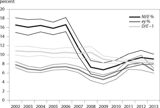
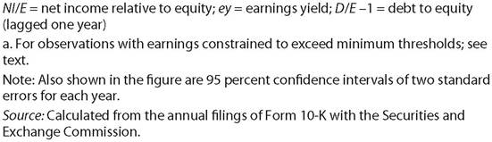
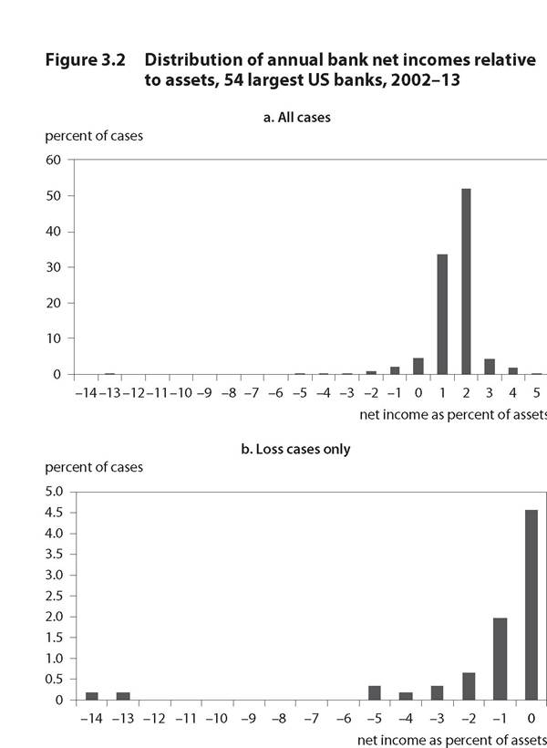
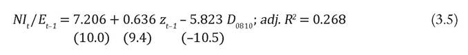
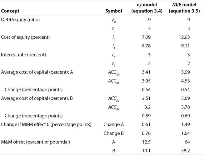
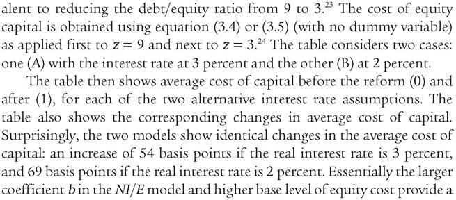
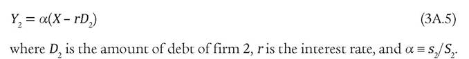
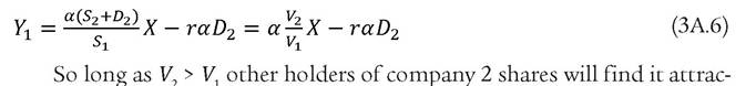
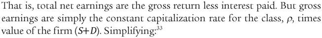
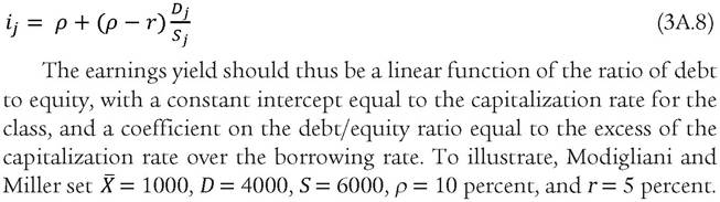
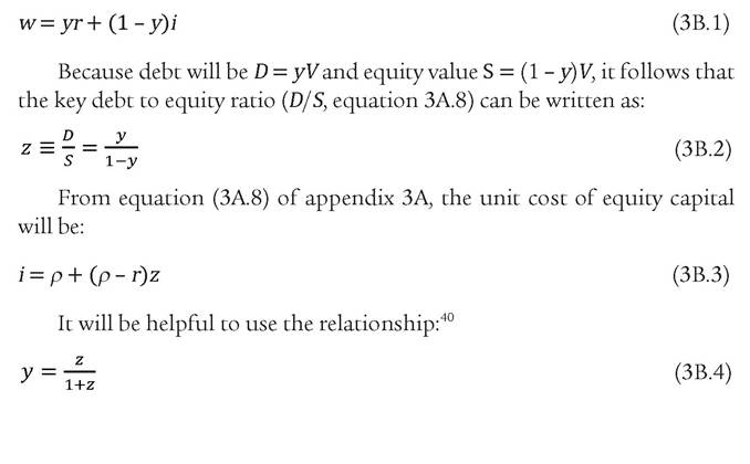
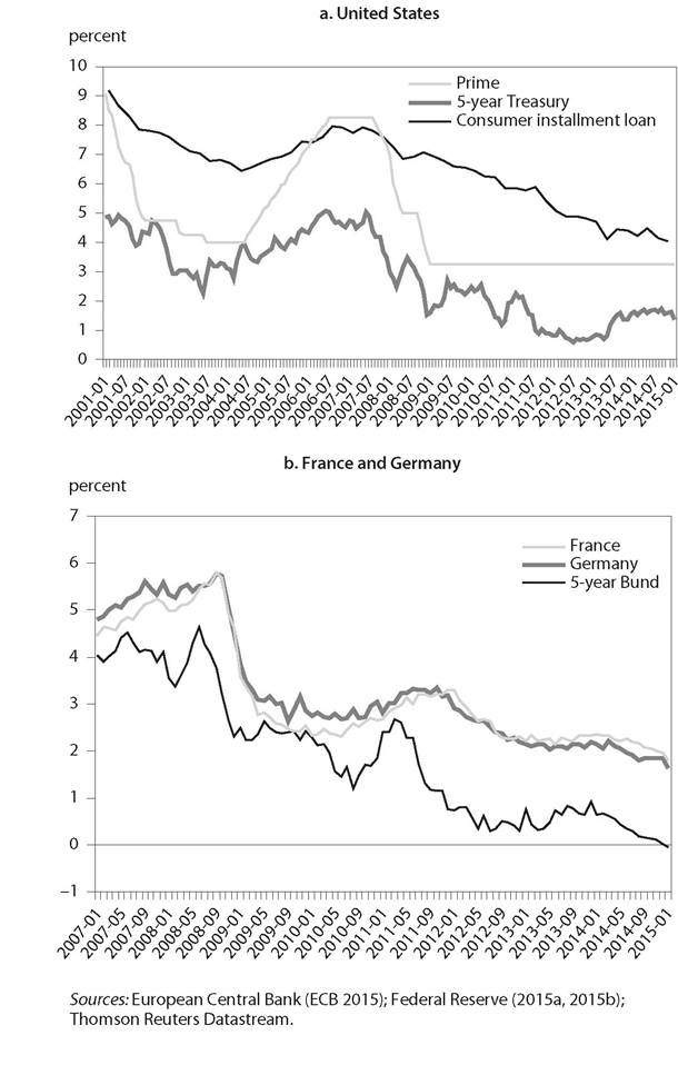
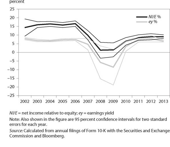
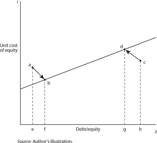
Like the banking crisis and Great Depression of the 1930s, the financial crisis and Great Recession of 2008-09 have provoked regulatory reform in the financial sector. Internationally, the new Basel III rules approximately double minimum capital requirements for most banks and triple them (or more) for systemically important financial institutions (SIFIs).[58] [59] The new requirements also introduce a minimum “leverage ratio” capitalization of 3 percent of total (as opposed to risk-weighted) assets under the Basel rules and 4 percent under US rules (BCBS 2014a, Federal Reserve 2013).[60] Some economists have called for far higher capital requirements. A key theoretical element of the argument of Admati and Hellwig and some other economists favoring far higher capital ratios is the “capital structure irrelevance” proposition of Modigliani and Miller (1958). The M&M hypothesis maintains that there is no optimal relationship of equity finance to debt finance for a firm, because any increase in profitability through greater leverage will be offset by an increase in the unit cost of the remaining equity capital as a consequence of greater risk. Based on this premise, some argue that there should in principle be no reason for banks to oppose far higher equity capital requirements because the resulting reduction in their leverage would result in a fully compensating reduction in the cost of equity capital.[61] In contrast, the few analytical attempts at identifying optimal capital requirements from society's viewpoint tend to acknowledge that higher capital requirements will make banks less profitable, and reduce lending and economic activity somewhat as a consequence. This chapter examines the empirical evidence on the M&M proposition as applied to the banking sector. It analyzes whether more highly capitalized banks do indeed enjoy lower costs of equity capital. The actual extent of such a relationship can then be used as an input into a broader analysis of optimal bank capital requirements from the standpoint of society, taking account of risks of financial crises from insufficient bank capitalization. Is Banking Special? At the outset it is useful to address in qualitative terms the question, “Why is banking different?” For the nonfinancial sector, shareholder equity capital typically accounts for about one-third of total assets, whereas debt and other liabilities amount to about two-thirds (see, e.g., Rajan and Zingales 1995, 1428). In contrast, in the postwar period US commercial banks have had equity-to-assets ratios (book value basis) of only 4 to 6 percent up to the 1970s, rising to 6 percent in the late 1980s and 9 percent by 2007 (Berlin 2011, 5). Leverage of debt to equity on the order of10 to 1 (or higher) instead of 3 to 1 has meant that the literature in this area has tended to treat the financial sector as “different,” typically excluding it from empirical tests. It seems intuitively appealing that the sector of financial intermediation should rely more heavily on debt financing than nonfinancial sectors. The intensity of inputs in a sector should depend on the nature of the output of the sector. One would not expect oil refining to have the same ratio of crude oil to total output as, say, the computer industry. Financial intermediation is a sector that by definition involves debt (in the form of deposits by households and corporations) as its main input. The main product provided by the bank is a store of value that has a high degree of safety and liquidity: bank checking and saving accounts. There is a considerable tradition in the literature that debt/equity characteristics of banking are likely to be different from those of other firms. Thus, in their analysis of equity returns Eugene Fama and Kenneth French (1992, 429) “exclude financial firms because the high leverage that is normal for these firms probably does not have the same meaning as for nonfinan- cial firms, where high leverage more likely indicates distress.” In a recent survey, Berlin (2011, 8) essentially adopts the proposition that financial intermediation is inherently levered when he states: “Since liquid liabilities are a primary output of the banking firm, we should expect banks to be highly levered.” Similarly, Herring (2011, 9) observes that “Since some liabilities are really a product supplied by the bank rather than simply a means of funding the bank, we know that a 100 percent equity-to-assets ratio cannot be the correct answer.” Although Miller (1995) himself informally discussed whether M&M applies to banking, his answer was an ambivalent “Yes and No” (the three-word abstract of his article).[64] One key reason that has been given for observed high leverage in banking is that deposits are subsidized by publicly provided deposit insurance (e.g., Admati and Hellwig 2013). Perhaps the most explicit analysis finding that banking is different is that by DeAngelo and Stulz (2013, 1, 3), who conclude that “MM’s leverage irrelevance theorem is simply inapplicable to banks... given a material market demand for liquidity, intermediaries will emerge to meet that demand with high leverage capital structures (made possible by asset structures optimized to produce liquidity).” In their model, with the bank choosing a portfolio of assets that is “not risky at the optimum” (p. 8), debt as a share of debt plus equity turns out to be the ratio 1∕[1+θ + φz]. Here θ is the “liquidity spread” that those purchasing liquidity from banks accept for assured future access to capital, φ is the “loan spread” paid on bank loans by those with limited access to capital markets, and z is the fraction of capital invested in loans that yield r (1 + φ), with the remaining fraction (1-z) invested in capital market securities at yield r. With reasonable values for θ and φ, this ratio will be high, relatively close to unity. Moreover, the contrast with lower bank leverage in earlier historical times can be explained by the bidding down of θ over time as financial markets developed. In a manner similar to the oil refining analogy suggested above, DeAngelo and Stulz (2013, 9) state that “Banks are different because financial flows are the inputs and outputs they utilize to generate value for their shareholders.” Calomiris and Herring (2013) also take issue with the notion that equity capital can be increased indefinitely without costs to the banks. Capital Assets Pricing Model Betas versus Direct Estimation It is important to emphasize that, unlike the few existing empirical estimates of the M&M effect for banks, the tests in this study do not use the indirect route of identifying the stock price “beta” for banks within the framework of the Sharpe-Lintner-Black capital asset pricing model (CAPM). In that framework, the riskiness of a given stock relative to a diversified equity portfolio is measured by the parameter beta, which tells the percent by which the stock price rises when the overall market rises by 1 percent, or falls when the overall market falls by 1 percent. However, it is much more direct to apply the estimation form implied by the original M&M article (as set forth in equation 3.1 below) than to infer the M&M influence through the bank beta in the CAPM framework. Such a test provides direct evidence on how much the equity yield can be expected to decline when the ratio of debt to equity is reduced. Because the CAPM has been found to provide poor explanation of equity prices with regard to the beta coefficient, it is problematic to rely on use of the beta as the indirect means to identify the M&M influence.[67] Fama and French (2004) find that the response of the equity return to changes in the stock's beta is only about one-third the size of what is predicted by the CAPM, such that stocks with low betas have higher than expected return and stocks with high betas have lower than expected returns.[68] On this basis, those who apply a bank beta estimated in relationship to leverage to calculate the reduction in required equity yields in response to higher capital should presumably shrink their raw estimates by two-thirds. At a broader level, it is curious to accept the CAPM beta framework to estimate how much additional bank capital would reduce equity capital cost without recognizing that the banking sector already has an average beta of about unity.[69] If bank stocks are already about as safe as the equity market as a whole, what are the grounds for arguing that the sector is unduly risky and needs deeper capitalization in comparison with other sectors? Arbitrage versus Optimization A final introductory remark concerns the framework of M&M and its relationship to other frameworks of optimization. At its core, M&M is based on a syllogistic arbitrage proposition: (1) Any debt-equity configuration chosen by the firm can be “unwound” by investors, who can sell shares of a highly leveraged firm and purchase shares in unleveraged firms using the proceeds plus borrowed funds, bidding down the share price of the leveraged firm and bidding up the share price of the unleveraged firm. (2) Market arbitrage will eliminate any profitability advantage of a more highly leveraged firm. (3) Therefore the capital structure (ratio of equity to debt) is irrelevant. Modigliani and Miller do not formally introduce risk. It is telling that their equations do not include an investor utility function, and they do not posit a typical degree of risk aversion. Nor do their equations set forth a probabilistic profile of returns in relationship to the debt-equity ratio, nor any hypothesized distribution function for returns. With such a function it would be possible to explore the optimal debt-equity ratio as a function of the risk aversion characterizing financial markets. Instead the authors appeal to “risk” only qualitatively and by implication maintain that any risk aversion whatsoever will suffice to drive their arbitrage process and rule out any superiority of one debt-equity ratio over any other. Specifying the Tests As set forth in appendix 3A, the M&M proposition leads to a straightforward specification for an empirical test: where i is the cost of equity capital as measured by ratio of earnings per share to price per share (the earnings yield or inverse of the price-to-earn- ings ratio); ρ is the “capitalization rate” at which expected streams of future earnings are capitalized (discounted) for the “class” (by implication, sector) of the firms in question; r is the rate of interest at which both the firm and investors can borrow; D is the firm's debt, and S is shareholder equity in the firm. Subscript j refers to the firm observed. Because the capitalization rate exceeds the interest rate (ρ > r), reducing debt relative to equity will reduce the earnings yield demanded by the market, thanks to reduction in perceived risk. The formulation turns out to cause exactly the amount of reduction in the earnings yield that is needed to have the average cost of capital remain constant. Moreover, this average cost of capital must equal the capitalization rate ρ (see equation 3A.4 in appendix 3A). The average cost of capital will be the weighted average of the cost of equity capital and the interest rate cost of debt. Defining V as the value of the firm, setting this value as being equal to debt plus equity (V= D + S ), and defining the debt financing share y as the fraction of total value attributable to debt rather than equity (such that y = D/V), it follows that: As demonstrated in appendix 3B, given equation (3.1), the derivative of ACC (average cost of capital) in equation (3.2) with respect to the ratio of debt to equity is zero. Capital structure (i.e., the decision to finance through debt as opposed to equity) therefore has no influence on the average cost of capital in the M&M framework. For purposes of empirical implementation, equation (3.1) can be estimated as: where z is defined as the debt to equity ratio (z = D/S), a = ρ, and b = (ρ - r). To support the M&M hypothesis, the constant a should be found to have a value that plausibly represents the return to capital in the banking sector (ρ), and the coefficient b should be such that a - b yields a plausible value for the interest rate r. Data The database developed for the tests in this study is drawn from the annual filings of form 10-K with the Securities and Exchange Commission for the 54 largest US banks, for the period 2001-13.[70] The asset sizes of the banks at the end of 2013 range from $6.5 billion for PacWest Bancorp (Los Angeles, California) to $2.4 trillion for JPMorgan Chase. The 54 banks had combined assets of $13.2 trillion at the end of 2013, representing 83 percent of total assets of US depository institutions (Federal Reserve 2014, 77) and about 75 percent of assets including the nondepository subsidiaries of bank holding companies (see chapter 7). The 10-K data report total assets, total liabilities, and shareholder equity (the difference). Total liabilities are used as the estimate of debt (D in equation 3.1), and shareholder equity as the estimate of equity (S ). The depen- dent variable i, cost of equity capital, is estimated as the inverse of the price- to-earnings ratio for the year in question, using the fourth-quarter average stock price and trailing 12-month earnings.[71] (For most banks, these data are from the 10-K filings and data for a few banks are from Bloomberg.) It is a standard principle of corporate finance that the “earnings yield,” or inverse of the price-to-earnings ratio, should be higher when the riskiness of the asset is greater.[72] There should be no ambiguity whatsoever that the “expected” earnings yield should be higher for higher risk, other things being equal. Ambiguity does arise, however, in measuring what investors expect future returns to be, because recently observed actual returns may or may not reflect those expectations. The price of a stock should be the discounted present value of its future stream of earnings. Expected future earnings depend on the base period earnings and the expected rate of growth of earnings in the future. The appropriate discount rate to apply equals the risk-free rate of return plus a premium to reflect the riskiness of the firm. In the M&M framework, this riskiness varies directly with the ratio of debt to equity. The discount rate will thus be higher for a more leveraged firm. Accordingly, for a specific class of firms (such as banks) in which the growth rate of future earnings is expected to be similar among the firms in question, the earnings yield is expected to be higher for firms with greater risk. Application of a higher risk premium in the discount rate will translate the future stream of earnings into a lower present value (stock price) relative to earnings. Although stock valuation is based on expected future earnings, empirical estimates require the use of actual observed earnings as the proxy for expected future earnings. However, use of the observed earnings yield as the measure of the cost of equity capital raises the problem of interpreting data for a year of losses. The problem is that in such years actual net earnings will not be a meaningful proxy for the expected stream of future earnings, the relevant concept in M&M. Investors would not supply capital if they believed future earnings would be negative, so by definition a year of losses does not provide a meaningful proxy of future expected earnings. Negative net earnings occur in about 8 percent of the bank-year observations, with heavy concentration (83 percent of negative instances) in the Great Recession years of 2007-10. The solution adopted here is to constrain the earnings yield observation to be no lower than the real return on US Treasury inflation-protected (TIP) five-year bonds, plus a risk spread of 100 basis points, as the lowest meaningful rate at which investors might be prepared to provide equity capital.[73] Choice of the real rate reflects the fact that when inflation is expected the nominal stream of earnings will be expected to rise over time, automatically providing inflation protection, such that inclusion of the inflation rate for the year in question would be doublecounting expected inflation. As an alternative measure of the cost of equity capital, a second test uses the ratio of net income in the year in question to the book value of equity at the end of the previous year. The same imposed floor replaces observations for years with negative income. Figure 3.1 shows the trends in the simple averages of these ratios for the 54 large US banks in 2002-13. The earnings yield (ey) refers to the inverse of the price-to-earnings ratio using trailing earnings and fourth-quarter average stock price, in percentage terms. Flanking confidence intervals at the 95 percent level for two standard errors for each year are also shown. Net income relative to equity (NI/E ) refers to net income for the year shown as a percent of equity (assets minus liabilities) at the end of the previous year, again in percentage terms. Both series are the constrained observations, overriding observations that are negative or too small as just discussed. The unconstrained series are shown in appendix 3D, figure 3D.1. They indicate average losses in 2008 and 2009 for the earnings yield measure and near zero averages for the net income relative to equity measure. Figure 3.1 also shows the ratio of debt to equity (lagged one year), this time as a pure number. It turns out that there has been significant deleveraging for US banks since 2007 (i.e., 2008 in the figure with respect to the debt/equity ratio). The ratio of debt to equity fell from an (unweighted) average of about 10.5 in 2007 to about 8 in 2013. Based on the same 10-K filings data, tier 1 capital is persistently an average of about 83 percent of book equity. By implication, the ratio of tier 1 capital to total assets rose from about 7.2 percent of assets to about 9.2 percent of assets over this period.[74] The (constrained) earnings yield, in contrast, has remained relatively steady within a range of 6 to 8 percent during this period, with the exception Figure 3.1 Net income relative to equity, earnings yield, and debt to equity ratio, averages for the 54 largest US banks: Constrained data, 2002-13a of a dip to as low as about 4 percent in 2009 in the Great Recession. However, the (constrained) ratio of net income to book equity capital has substantially declined, from about 16 percent to a range of 8 to 10 percent. The contrast between the income-book equity ratio and the earnings yield is a manifestation of the decline in the ratio of market capitalization to book value of equity, which fell from an average of 2.26 in 2001-06 to 1.23 in 2007-09 and 1.15 in 2010-13 (market capitalization data are from Bloomberg). It is informative to consider the distribution of net income for these large banks over the 12-year period 2002-13. Figure 3.2 is a histogram showing the distribution of net income as a percent of total assets at the end of the previous year. The first panel shows the full distribution. The second panel shows the distribution for just the cases of losses. In the second panel, the right-hand bucket “0” refers to the percent of bank-year observations with net income between -1 percent and zero. A total of 8.3 percent of bank- year cases had negative income in this period (which included the worst Sources: Calculated from annual filings of Form 10-K with the Securities and Exchange Commission and Bloomberg. recession since the 1930s). Only 1.1 percent had losses exceeding 3 percent of assets (the new Basel III capital leverage standard) and only 0.7 percent had losses exceeding 5 percent of assets (the US largest-bank capital leverage standard). Critics of the low Basel ratio often seem to consider it self- evident that the 3 percent level is far too low given the losses that might be expected, but it turns out that the frequency of larger losses is relatively low. Of course, a major caveat is that book income may be overstated (and losses understated) by failing to capture erosion in market value of assets in periods of stress.[75] Nonetheless, the distribution of income results in figure 3.2 suggests that setting the capital leverage ratio far higher than the US level would amount to addressing a small fraction of cases based on the most recent decade's experience. Test Results The tests here estimate equation (3.3) using a pool of 12 years' observations on 51 of the 54 largest US banks.[76] Because of the unusual conditions during the Great Recession, the tests include a dummy variable for the years 2008-10. For the earnings yield variant of the unit cost of equity capital, the results are:[77] where ey is the earnings yield (percent), or inverse of the price-to-earnings ratio; z is the ratio of debt to equity (with equity defined as the excess of book assets over book liability); and D is a dummy variable with value 1 for 2008-10 and 0 otherwise. T-statistics are in parentheses. The coefficient on the leverage ratio is not significant. Importantly, the size of the coefficient is relatively small, about 5 basis points for each unit change in the leverage ratio. Instead, the M&M value for the coefficient should be ρ - r. It seems unlikely that the interest rate r would be so close to the bank “class” rate of return on capital that the difference would be this small. When the net income/equity variant is applied instead as the measure of the unit cost of equity capital, there is a considerably stronger relationship: where NIt /Et1 is the ratio of book net income to equity at the end of the previous year (percent). This time the coefficient on the leverage ratio is highly significant. Moreover, its size is substantial, at about 60 basis points for each increment by unity in the ratio of debt to equity. Nonetheless, even this magnitude is small as a likely gauge of the excess of the banking sector return on capital minus the interest rate. Application of fixed-effects tests for an unbalanced panel yields results that are very close to those of equations (3.4) and (3.5).20 Because of their simplicity and transparency, the results in equations (3.4) and (3.5) are applied in the impact estimates below. A potentially important statistical question is whether the estimates are biased because of endogeneity. It could be argued that treating the capital ratio as an exogenous right-hand-side variable misses the point that investors might put pressure on a highly leveraged bank to raise its capital. If they do, the observed capital ratio might already reflect some moderation prompted by market forces.[78] [79] Appendix 3E investigates this question. It concludes that if such endogeneity does exist, the measured M&M coefficient (b in equation 3.3) should not be affected (and hence is unbiased) even though the observed range of variation in debt leverage would be smaller than the ex ante range.[80] Implications for the Average Cost of Capital Table 3.1 considers the implications of a sharp increase in bank capital requirements on the average cost of capital for banks. The table uses the estimates in equations (3.4) and (3.5) to assess the effects of raising bank capital from a benchmark of 10 percent of total assets to 25 percent (the midpoint of the range suggested by Admati and Hellwig 2013). This increase is equiv- Table 3.1 Impact of raising the capital-to-assets ratio from 10 to 25 percenta ey = earnings yield; M&M = Modigliani and Miller; NI/E = net income/equity a. Refers to total assets, not risk-weighted. Source: Author's calculations. [1] That is, with the shares of D and E, respectively, at 0.9 and 0.1, D/E = 0.9/0.1 = 9. With these shares instead at 0.75 and 0.25, D/E = 0.75/0.25 = 3. [1] The value for b estimated in equation (3.4) is applied even though it is not significantly different from zero. substantially larger absolute reduction in the cost of equity, but because the equity cost (both before and after) is substantially higher in the NI/E model than in the equity yield model, there is a fully offsetting effect from a more powerful impact of shifting from low-cost debt to high-cost equity. The table next shows the change in average capital cost that would occur if there were no M&M effect at all (namely, the unit cost of equity capital after the reform is identical to that before the reform). Finally, the table reports the corresponding percent of total potential increase in average cost of capital that is offset by the induced reduction in equity capital cost as a consequence of the M&M effect. As expected from the small size of coefficient b in the ey model and large size of this coefficient in the NI/E model, the percentage offset is much smaller in the earnings yield model (only about 10 percent) than in the net-income model (about 60 percent). Taking the averages over the two models and two alternative interest rates, the expected change in the average cost of capital from the higher capital requirement would amount to 61.5 basis points. In the absence of any M&M offset the average increase would be 112.5 basis points. So on average, the M&M offset amounts to 45 percent of the potential increase in the weighted-average cost of capital.[81] Banks could be expected to pass along the net increase to household and corporate borrowers. Permanently higher real interest rates would reduce the amount of capital formation and thus reduce future GDP from levels otherwise reached. The central estimate, an increase of approximately 62 basis points in average cost of capital for an increase in capital of 15 percent of total assets, is considerably more modest than would be implied by the findings of Cohen and Scatigna (2014) for actual behavior of lending rates so far during the phase-in of Basel III. They estimate that for a sample of 94 banks in both advanced and emerging-market economies, common equity capital rose from 11.4 percent of risk-weighted assets in 2009 to 13.9 percent in 2012 (p. 12). Net interest income rose from 1.37 percent of total assets to 1.67 percent. The authors state that the 30 basis point increase translates to 12 basis points per percentage point increase in the (risk-weighted) capital- to-assets ratio. Considering that risk-weighted assets would likely be no more than 50 percent of total assets going forward (the 2012 ratio was only 0.42; p. 11), each percentage point of total assets increase in capital would impose at least 24 basis points increase in lending cost based on the Cohen- Scatigna results. In the exercise of this study, the 15 percentage point increase in capital relative to total assets would thus boost bank lending costs by 360 basis points. So the estimates here can be seen as substantially on the conservative side in comparison with actual experience under increased capital requirements in 2009-12. Similarly, the increase of 62 basis points estimated here is more modest than the corresponding increase implied by the estimates of Miles, Yang, and Marcheggiano (2012), which would amount to 81 basis points for the same increase in capital. As discussed in appendix 3C, they estimate that raising capital by 3.33 percent of total assets (reducing the asset/capital leverage ratio from 30 to 15) would increase the weighted-average cost of capital by 18 basis points after taking account of the M&M offset (induced reduction in equity cost). Applying an increment of 15 percentage points of assets would thus imply an increase of 81 basis points (= 18 ? [15/3.33]). Another study discussed in appendix 3C, by Yang and Tsatsaronis (2012), obtains results that imply a 15 percentage point increase in the ratio of capital to total assets would boost the weighted-average cost of capital by 120 basis points. The findings of these two studies thus also imply that the estimates in the present study for the impact on lending rates from a 15 percentage point increase in capital relative to assets may be understated rather than overstated, although not by as wide a margin as implied by comparison to the findings of Cohen and Scatigna (2014) for increases that have already occurred from the much smaller capital increases as a result of the initial phase-in of Basel III. Lower Borrowing Cost for Banks? The original M&M analysis held all unit costs of debt fixed. But some authors emphasize that higher equity capital would reduce unit borrowing costs for banks as well. The reason would be the same as that for equity: Creditors (as well as equity investors) would perceive less risk than before. Gambacorta and Shin (2016) examine the borrowing cost question using data for 105 international banks in 14 advanced economies over the period 1995-2012. They conclude that a 1 percentage point increase in the ratio of equity to total assets reduces the average cost of bank debt funding by 4 basis points. The authors use an example in which equity capital is raised from 5.6 percent of total assets to 6.6 percent, equity unit cost is held constant at 10 percent, and debt unit cost is 3.1 percent. Whereas a “naive” direct calculation shows an increase of 7 basis points in average cost of total funding, the net increase is only 3 basis points after applying their estimated regression coefficient to calculate the reduction in unit cost of debt.[82] A problem with their presentation, however, is that they neglect to point out that the same exercise yields a far smaller impact if the empirical estimate for the most directly comparable alternative specification in their tests is applied instead.[83] Although more research examining the impact of capital on borrowing cost would seem warranted, the main basis for analyzing the economic cost of higher capital requirements remains the M&M influence on equity cost. Conclusion The M&M offset is a key building block in any analysis of the optimal capital requirement for banks. The central finding of this chapter is that this offset parameter is 0.45. Namely, although equity capital has a higher unit cost than debt, slightly less than half of the increase in average unit cost of capital to banks that would otherwise result from raising bank equity capital requirements as a consequence of this differential is offset by the reduction in the unit cost of equity capital demanded by investors, thanks to the reduction in risk provided by the reduction in leverage. The calculations of chapter 4 apply this value for the M&M offset parameter in arriving at estimates of optimal capital requirements. Appendix 3A The Modigliani-Miller Model Modigliani and Miller (1958, 267-71) posit that for any given “class” of firms (implicitly, for example, a particular industrial sector), in the absence of any debt financing the price of a share of a given firm j will be the expected annual stream of income earned (“expected return”) discounted by the expected rate of return for that class. Thus: returns (earnings, abstracting from taxes) per share, and ρ is the characteristic rate of return to that class of firms.[84] They then introduce debt financing and examine its influence on share pricing. Their first proposition is that “the market value of any firm is independent of its capital structure and is given by capitalizing its expected 1. 1 shares, X is expected return on assets owned by the company (before deduction of interest), and Dj is the market value of the debt of the company.[85] The authors define the “average cost of capital” as the ratio of expected return to the market value of all the firm's securities. Their proposition is then that this average cost is constant at the rate ρ applicable to the class in question, and consequently is “completely independent of the capital structure and is equal to the capitalization rate of a pure equity stream of its where ACC is average cost of capital (my addition). This proposition challenged the then dominant view that average cost of capital was a declining function of leverage until leverage reached so high that the average cost rose once again because of rising risk, with the implication that there was some optimal leverage ratio.[86] The conventional view apparently reflected the sense that debt capital was cheaper than equity capital so higher leverage would reduce the average cost of capital, whereas the central proposition of M&M was that higher leverage would introduce higher risk and increase the cost of equity capital enough to offset the rising share of debt capital. To demonstrate this proposition, the authors invoke arbitrage between the share prices of two firms, one leveraged and the other not. Both firms have the same expected return (gross of interest), stated thus as simply X. The authors first suppose that the value of the levered firm, V2, is larger than that of the unlevered one, V1. They then consider an investor holding s2 dollars' worth of shares in firm 2, constituting the fraction α of total shares in the firm worth S2. The return to this investor, Y will be the owned fraction of the firm times its income net of interest costs, or: The authors next have the investor sell his αS2 worth of shares in company 2 and purchase the larger amount s1 = α (S2 + D2) of shares in company 1. In doing so, the investor borrows the amount αD2 to supplement the proceeds of the sale of company 2 shares. Keeping in mind that in firm 1 there is no debt so the value of the firm is solely total equity share value S1, the investor's income from the new holding in company 1 net of interest paid on the amount borrowed is then: tive to imitate the first investor, because Y1 (equation 3A.6) will exceed Y2 (equation 3A.5). This process will bid up the price of company 1 shares and bid down the price of company 2 shares until V2 = V1. The authors conclude “levered companies cannot command a premium over unlevered companies because investors have the opportunity of putting the equivalent leverage into their portfolio directly by borrowing on personal account” (p. 270). Of course, this conclusion requires that the outside investors can borrow at the same interest rate as that paid by company 2 on its debt, “r”. It is not clear in general that this would be the case; certainly retail investors seem likely to pay higher interest on stock margin debt than the typical borrowing cost of a sound firm. For banking, it is even more unlikely that outside investors can borrow at the same rate, because one-half or more of the funding of the bank is likely to come from deposits that bear extremely low interest rates (if any). One can thus begin to see limitations on application of the model, especially for banks.[87] Modigliani and Miller then show that conversely, if the unlevered firm were more valuable than the levered firm, the investor in the unlevered firm could sell stock, use the proceeds to buy shares in the levered firm and invest what is left over in bonds, until the value of the levered firm were bid up to that of the unlevered firm. This process would amount to “an operation which ‘undoes' the leverage” (p. 270). However, the general presumption had been that if there were any difference, levered firms would be more valuable, so the algebra going in the opposite direction need not detain this appendix. The authors then turn to the result that is key for the empirical test here: The earnings yield of the stock in question should equal the capitalization rate appropriate to the class of the firm plus a constant times the ratio of debt to equity. The constant in question is the excess of the capitalization rate over the interest rate. This result is derived as follows. The earnings yield on a share of the stock will be:[88] [89] Expected yield or rate of return per share is then 13.3 percent.[90] In their example, if the capital structure reverses from 60 percent equity to 40 percent equity, the earnings yield should rise from 13.3 to 17.5 percent.[91] This linear relationship of earnings yield to leverage (defined as the debt-equity ratio) holds the average cost of capital constant regardless of leverage. Thus, in the first case capital costs an average of 0.4 ? 0.05 + 0.6 ? 0.133 = 0.1, or 10 percent. In the second case, capital costs an average of 0.6 ? 0.05 + 0.4 ? 0.175 = 0.1, again 10 percent. In the case of US banks, with equity capital at about 10 percent of total assets and thus the debt-equity ratio at about 9, these same postulated rates would place the earnings yield implausibly high at 55 percent (and the price-to-earnings ratio implausibly low at 1.8). Instead, at the end of 2014 the median trailing price-to-earnings ratio for the seven largest US banks was approximately 16, placing the earnings yield at about 6 percent.[92] For the same banks, the median credit default swap (CDS) rate spread above 5-year US Treasury bonds in 2013 was 78 basis points, placing the corresponding borrowing rate at 2.73 percent.[93] By implication equation (3A.8) would require that the bank sector capitalization rate (ρ) was only 3.06 percent.[94] This capitalization rate is implausibly low, however. By implication, the sensitivity of the earnings yield to leverage may be overstated by the M&M model. Appendix 3B Demonstrating Constant Average Cost of Capital in Modigliani and Miller The original equations in Modigliani and Miller (1958) show a clear negative relationship between the unit cost of equity and the amount of debt leverage. The authors use a numerical example to demonstrate that as a consequence the average cost of capital is constant and does not depend on leverage. It is useful to show that this result is general for their setup. Especially for banks, with high leverage, the ratio of debt to equity might be thought to have nonlinear consequences for the average cost of capital as leverage rises even higher, if only because in the limit this term (the final variable in equation 3A.8, appendix 3A) would approach infinity.[95] This appendix shows that the derivative of the average cost of capital with respect to the debt/equity ratio is zero, demonstrating that the result of constant average cost of capital is general. Define w as the average cost of capital, and y as the ratio of debt to total enterprise value. (In the terms of appendix 3A, y = D/V = D/ (D + 5).) With the interest rate at r and the cost of equity capital at the rate i (and with i in turn equal to the net earnings yield per share), average cost of capital will be: [1] Their numerical example involves intermediate levels of leverage, with the debt to equity ratio rising from only 2/3 to 1.5, well below the range observed in the banking sector. Appendix 3C Alternative Analyses of the Modigliani-Miller Offset for Banks As discussed in chapter 2, there is a surprisingly wide divergence of expert opinion on the costs of increasing bank capital requirements (let alone on the social benefits). Several academic studies tend to invoke the M&M theorem as grounds for judging these costs to be minimal. The official sector studies have tended to quantify costs without explicit allowance for the M&M offset (lower cost of equity capital thanks to less risk as leverage declines) but with qualitative recognition of the potential offset. One important industry study, in contrast, took note of the theorem but rejected it and arrived at relatively high costs of increased capital requirements. This appendix examines both that study (IIF 2011) and three leading papers on the other side of this spectrum to shed further light on the debate. The literature survey in appendix 2A provides a summary of an important study by the Institute of International Finance (IIF 2011). Whereas that study had predicted a sizable increase in bank lending rates and spreads above risk-free rates for the period 2011-15 as a consequence of the phasing in of Basel III capital requirements, such increases did not occur, as shown in figure 3C.1. In panel A for the United States, the spread between the prime rate and the 5-year US Treasury rate was an average of 362 basis points in 2007, fell to an average of 173 basis points in 2011, and instead of rising fell slightly further to 163 basis points for 2014 and early 2015. The corresponding spreads for consumer installment loans averaged 334, 429, and 262 basis points, so on this measure, from 2011 to 2014-15 the lending cost to private borrowers relative to the risk-free benchmark fell rather than rising.[96] In panel B for France and Germany, interest rates for new bank lending to nonfinancial corporations are shown, along with the 5-year rate for the German treasury bond. The average spread for the two countries above the 5-year German bund did edge up, from 130 basis points in 2011 (already up from 89 basis points in 2007) to 173 basis points in 2014-January 2015. The increase of 43 basis points from 2011 to 2014-15 is consistent with some impact of higher capital requirements on lending rates, but far less than had been projected in the IIF study.[97] Figure 3C.1 Bank lending rates in the United States and euro area, 2001-15 Miles, Yang, and Marcheggiano (2012) conduct tests for 7 UK banks for the period 1997-2010 to estimate the influence of leverage on the cost of equity capital. They apply the CAPM framework and thus focus on estimating market betas rather than directly investigating the relationship of equity yield to leverage. In their main finding, the equity beta equals a constant 1.07 plus the estimated coefficient 0.03 times the ratio of assets to capital (pp. 10, 13). With an average asset to capital ratio of 30, by implication the average beta was approximately 2.46 They translate the implications for equity cost of higher capital requirements as follows. They place average return on equity at approximately 15 percent, average bank borrowing cost at 5 percent, and average leverage at 30, implying weighted-average cost of capital (WACC) of 5.33 percent.[98] [99] [100] They then consider the impact of doubling required capital, or lowering the leverage ratio from 30 to 15. In the absence of any M&M offset the effect would be to boost WACC to 5.66 percent, an increase of 33 basis points.[101] The authors then calculate the impact of higher capital requirements taking account of their estimated M&M offset. In the CAPM, the equity cost of a firm equals the risk-free rate plus the firm's beta multiplied by the market average risk premium. They place the risk-free rate at 5 percent, and the general market risk premium at 5 percent. With their regression estimate, the cost of equity capital at the lower leverage ratio (15 instead of 30) would fall to 12.6 percent.[102] As a consequence, the new WACC would be 5.51 percent.[103] The rise in the WACC would be 18 basis points instead of 33, indicating that the M&M effect would offset 45 percent of the potential rise in average cost of capital. As it turns out, the central estimate in this study is also that the M&M offset would be 45 percent of the potential rise in the average cost of capital for bank lending. That estimate involves a more ambitious increase in capital (reducing the asset to capital ratio from 10 to 4, rather than from 30 to 15). Finally, the authors acknowledge that the alternative of directly testing the relationship of required return on bank equity to bank leverage “has the advantage of not assuming the CAPM holds” (p. 14). Unlike the present study, they find that in a regression of realized earnings relative to price (the equity yield) on leverage, “the impact on the required return on equity of changing leverage is about as big as if MM held exactly” (p. 15). Unfortunately, they do not report these results.[104] Yang and Tsatsaronis (2012) use a CAPM framework incorporating leverage as a shift variable affecting estimated betas. They find a statistically significant influence of leverage on the cost of equity capital. However, this influence turns out to be relatively small. The estimates indicate that “if the ratio of a bank's total assets to its equity increases by 10 and the market return is 4 percent in excess of the risk-free rate, the bank pays 0.4 percent more for every unit of equity” (p. 51). Correspondingly, the authors calculate that if average leverage fell from 20 to 10, the cost of equity capital would fall from 13.4 to 13.0 percent. Taking into account a 5 percent cost of debt, the weighted-average cost of capital would rise from 5.4 to 5.8 per- cent.[105] The M&M offset in the study by Yang and Tsatsaronis is also relatively small. With no induced change in the cost of equity capital, doubling equity from 5 to 10 percent of total assets would raise the average cost of capital from 5.42 to 5.84 percent, an increase of 42 basis points. After taking account of induced reduction in the cost of equity capital, the average cost of capital would still rise to 5.80 percent, a net increase of 38 basis points.[106] The M&M offset from induced reduction in the equity rate would thus be only 4 basis points, or about one-tenth of the increase at ex ante returns. The main text above instead places the offset at about 45 percent. An increase of 40 basis points in the average cost of capital for an increase in capital of only 5 percent of total assets, moreover, would imply an increase in average cost of capital of 120 basis points for a capital increase amounting to 15 percent of total assets, the exercise considered in the main text here. This increase would be considerably larger than the corresponding increase of 62 basis points estimated in the main text. In another study employing the CAPM framework for US banks, Hanson, Kashyap, and Stein (2010) estimated that the long-run steady-state impact of higher capital requirements on lending rates should be modest, only 25 to 45 basis points for a (large) 10 percentage point increase in capital relative to total (not risk-weighted) assets. They noted, however, that short-run frictions associated with raising capital could be substantial, implying the need for gradual phase-in. They also suggested increased regulation of the shadow-banking sector to avoid increased fragility in the system as a consequence of possible migration of financing out of banking in response to higher capital requirements. The authors regress bank betas on the capital-to-assets ratio for US banks in 1976-2008. They find a significant coefficient of -0.045. With the median bank beta at 0.90 and capital-to-assets ratios at a median of 7 percent, they argue that this finding is “broadly in line with what is predicted by the [M&M] conservation-of-risk principle” (p. 17). Namely, doubling capital to 14 percent of assets would reduce the beta by 0.32 (= 0.045 ? 7) to a level of 0.58, not far from the level of 0.45 that would be half the original median beta. However, they do not formally demonstrate that the original M&M formulation should translate to a reduction in bank market beta proportionate to a reduction in the assets-to-capital ratio.[107] The authors apply a prior assumption of strong M&M effects to calibrate the impact of higher capital requirements on lending rates. In their preferred variant, the effect is complete except for the distortion from corporate tax deduction for interest but not dividends. They estimate this effect as causing a 25-basis-point increase in the lending rate as a consequence of 10 percent of assets in additional capital. With a corporate tax rate of 35 percent, the effect of shifting this amount of finance from debt to equity, even with induced reduction in the unit cost of equity, would be 0.35 ? 700 ? 0.1 = 25 basis points. The upper bound of their range adds another 10 basis points for loss of convenience of short-term debt as well as a further 10 basis points catch-all for all other violations of M&M (“arbitrary fudge factor,” p. 18), to arrive at a maximum 45-basis-point increase in the bank lending rate (for a 10 percentage point increase in the capital-to-assets ratio). Surprisingly, the authors do not specify the ex ante equity capital cost. They do cite a debt cost of 7 percent (which seems high, certainly for a real concept that should be used for comparison to equity). By implication, if they considered the equity cost to be 14 percent ex ante, then in the absence of any M&M effect at all the total increase in weighted-average cost of capital would be 70 basis points.[108] The authors thus implicitly judge that the M&M offset amounts to at least 36 percent of the otherwise potential increase in lending cost ([70 - 45]/70) and, in their preferred estimate, as much as 64 percent ([70 - 25]/70). The authors further seek to show that lending rates have not been influenced much by capital-to-assets ratios in the past (from the 1920s to the present), but their message is somewhat clouded by the fact that of their three alternative measures the only one with a statistically significant coefficient on the capital-to-assets ratio must be rejected out of hand because it indicates an excessively large increase in lending cost for a given rise in capital. Despite their strong prior on full M&M effects, the upper end of the range identified by the authors is surprisingly similar to the estimate of the present study. The lending-cost impact for 15 percentage points of assets in additional capital would be 67.5 basis points (applying their upper-bound 4.5 basis points per percentage point increase in the capital-to-assets ratio), slightly above the 62 basis points estimated in the main text of the present study. Appendix 3D Trends in Unconstrained Earnings Indicators of the Cost of Equity Capital The tests in the main text constrain observations on equity yield and net income relative to equity to be positive. For cases where earnings are negative, these two proxies for cost of equity capital are constrained to be greater than zero and are set equal to the real 5-year Treasury bond rate plus a moderate spread, as discussed in the main text. Figure 3D.1 shows the paths of the averages for the 54 banks using the unconstrained data, whereas figure 3.1 in the main text shows the constrained data. Confidence intervals (5 percent level) for each year are shown as well. Figure 3D.1 Net income relative to equity and earnings yield, averages for the 54 largest US banks: Unconstrained data, 2002-13 Appendix 3E Possible Endogeneity Bias Suppose that a risk-averse bank plans on an ex ante basis to employ debt to equity leverage z represented by the horizontal distance at point “a” in figure 3E.1, and expects to have to pay the unit cost for equity i represented by the vertical distance at that point. Suppose a risk-prone bank plans to employ corresponding debt/equity leverage shown by the horizontal distance to point “c”, anticipating equity unit cost of the vertical distance at that point. Now consider the influence of “market pressure” on equilibrium positions. The endogeneity proposition is that investors will press the risk-prone firm to be more cautious (reducing z) and even then will require higher unit equity cost than the firm had sought (raising i), shifting the firm's position to point “d”. Similarly, investors considering the plans of the risk-averse firm will admonish it to be more aggressive (boosting z) and even so are willing to provide equity at lower unit cost than the firm had anticipated (reducing i), moving the firm to the somewhat more risk-prone position at point “b”. Figure 3E.1 Relationship of unit cost of equity to debt-to-equity ratio What will be the consequences of this endogeneity for the measured relationship of unit cost of equity to the observed debt/equity leverage? The initial positions a and c have no meaning because the market would not make equity available at the ex ante terms expected by the firms. The meaningful relationship will be shown by the line bd. The M&M proposition is that there is a linear relationship between unit cost of equity and debt/equity leverage, so the empirical measurement process should not be distorted. It is completely another matter whether the resulting measured line cd has a sufficiently steep slope that the M&M offset is complete. The findings in equations (3.4) and (3.5) indicate not. But there should be no bias in the observed slope from the influence of the narrowing of the range of variation of the debt/equity leverage resulting from endogeneity to market pressures, so long as the relationship is linear as posited in M&M. The induced reaction of banks in moving from a to b and from c to d does narrow the range of observed variation in debt leverage. The observed range will be distance fg instead of distance eh for ex ante leverage. Nevertheless, in the US bank data there remains a wide range of variation in observed leverage. Thus, for the full period in the estimates of equations (3.4) and (3.5), the bank at the 12th percentile showed an average debt/ equity ratio of 6.0 whereas the bank at the 88th percentile had an average debt/equity ratio of 13.1.


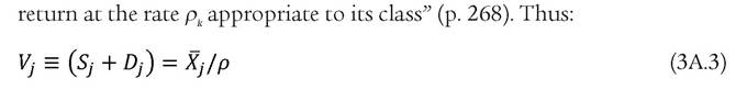 where V. is the market value of the firm, S. is the market value of its common
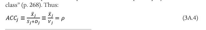

More on the topic Testing the Modigliani-Miller Theorem of Capital Structure Irrelevance for Banks:
- Testing Modigliani-Miller for Banks
- References
- Cline W.. The Right Balance for Banks. Peterson Institute for International Economics,2017. — 281 p., 2017