Chapter 70 International Portfolio Diversification Benefits among Developed and Emerging Markets within the Context of the Recent Global Financial Crisis
Gulin Vardar
Izmir University of Economics, Turkey
Berna Aydogan
Izmir University of Economics, Turkey
Ece Erdener Acar
Izmir University of Economics, Turkey
ABSTRACT
This chapter aims to examine the existence of dynamic linkages among the major emerging stock markets, namely Brazil, Hungary, China, Taiwan, Poland, and Turkey, as well as developed markets, particularly the US, the UK, and Germany during the period 2004-2013.
Potential dynamic long-run interdependencies are investigated using Johansen and Juselius (1990) multivariate cointegration test and causal relationship through the Vector Error Correction Model (VECM). Moreover, to capture the impact of the recent global crisis on the cointegrating relationship among the developed and emerging markets, the sample period is divided into pre- and post-crisis sub periods. The empirical findings show that, after the crisis period, the direction of the long-run relationship varies, and furthermore, the stock market interdependence increases, supporting herding behavior of investors during the stock market crash period. Therefore, the increasing dynamic co-movements in the period after the crisis provide direct implications for the international investors due to potential limitation in the international risk diversification and the achievement of greater portfolio returns through global investment.DOI: 10.4018∕978-1-4666-6268-1.ch070
.
INTRODUCTION
Portfolio management, in general sense, is the design of optimal portfolios that match the rational investor’s objectives with the future prospects of portfolio manager. Modern portfolio theory states that investors constantly attempt to maximize the expected rate of return through diversification opportunities. The increasing trend in the free capital flows, technological developments in communication and trading systems, thereby, reduction in cost of information and the introduction of new financial products create more diversification opportunities for both individual and institutional investors.
Rational investors make their decisions based on their risk aversion rather than maximizing the expected utility. Therefore, international investors have begun to implement international portfolio diversification as a tool for reducing the expected portfolio risk and maximizing the expected rate of return.One of the main principles of international diversification is the existence of uncorrelated return among markets. When returns from investments in different countries’ stock markets are not correlated, the opportunities generated from portfolio diversification are more profitable, according to modern portfolio theory (Elton & Gruber, 1995; Farrell, 1997, Strong, 2000). In recent years, however, globalization, economic and financial integration and assimilation between countries have enhanced the interdependency of global markets and these phenomena seem to affect the decisions of investors in the allocation of financial assets. It is well accepted that integration of financial markets, is primarily linked to economic growth through risk sharing benefits, improvements in allocation efficiency, and reductions in macroeconomic volatility (Pagano, 1993). Since greater integration exists between national stock markets, investors prefer to make an investment in the emerging markets to exploit benefits of international diversification, in the belief that there may be low correlations between developed and emerging markets. In this context, reflecting the trend towards greater integration of stock markets, this chapter explores how application of international portfolio diversification occurs among developed and emerging markets through an assessment of the impact of recent global financial crisis.
The recent global financial crisis is entitled as one of the most severe, because of its global nature. The crisis started in the US and spread through major stock markets all over the world, leading to confusion among policy makers and investment practitioners, and raising many questions relating to the subject of international financial integration.
Characterized by turbulent financial markets and widespread economic slowdown across the countries since the middle of2007, this crisis could be fuelling entirely negative impacts on international financial integration. Given that significant changes have occurred across the world financial markets, it appears timely and interesting to examine whether the relationships among these markets have changed over this crisis period. Therefore, understanding the interaction of global markets across countries interact could provide crucial inputs for policy purposes in dealing with crises spreading from one country to another.This chapter concentrates on the following questions:
1. What is indicated by any dynamic long-run relationship among emerging and developed stock markets over the period?
2. Have the long-run relationships across stock markets changed since the recent global financial crisis?
3. What are the short-run linkages and causality effects between major developed and emerging stock markets over the period?
4. Are there any specific changes in the shortrun and causal relationship among the sample countries after the recent global crisis?
5. How does the recent global crisis affect the integration of emerging and developed stock markets’?
6. What are the key implications of the recent global financial crisis on stock market integration?
Based on the questions above, this chapter investigates possible long-run relationship and short-run dynamic causal linkages between major stock markets in developed countries, particularly the US, the UK and Germany, and those in emerging countries, namely Brazil, Poland, Hungary, Taiwan, China and Turkey, during the period 2004-2013, and also assesses the impact of the recent global financial crisis on the level of financial integration among these markets. This study is of particular importance for both investors and corporate managers, as it considers the influences on international asset allocation and diversification benefits and the cost of capital, which contribute significantly to economic growth.
The contribution of this chapter to the literature is two-fold: First, it utilizes a comprehensive data set that includes daily data for the major stock markets of developed and emerging countries from April, 2004 to March, 2013. Second, it considers whether the recent global financial crisis has resulted in long and short-term structural changes on the co-integrating and lead-lag relationship among the stock markets. To the author’s best knowledge, it would appear that a limited number of studies have addressed the issue of how this crisis altered market integration among these countries. By dividing the sample into two sub-periods, it also considers potential differences in terms of international diversification benefits available for both institutional and/ or individual investors before and after the recent global financial crisis.
The rest of this chapter is organized as follows. The first part focuses on broad definitions and discussions of the topic within the scope of literature. The second part outlines the econometric methodology, followed by data set. The third part presents the empirical results. Future research directions are discussed in the fourth part. Finally, the chapter concludes with discussion of the overall coverage.
BACKGROUND
The study of Markowizt (1952) is esteemed as first to quantify portfolio diversification, and pioneered the concept of modern portfolio theory. There is always a tradeoff between risk and return in the field of investment. Basically, if an investor invests in an asset with high expected return, the expected risk would be higher for that asset as well. Modern portfolio theory is in the center of this tradeoff, and describes how to select a portfolio that would maximize the expected return through diversification opportunities. Starting from 1970s, liberalization trend in international stock markets led to international investment movements which encouraged international portfolio diversific ation (Haroon et al., 2012).
The primary motivation for international portfolio diversification is to reduce the expected portfolio risk and expand the opportunities for expected portfolio return beyond those available through domestic securities. Investors are assumed to be risk averse in classical portfolio theory, thus they search for an optimal portfolio that maximizes the expected utility (Fama & MacBeth, 1973).The total risk of any portfolio is composed of two types, systematic, referring to market risk, and unsystematic, referring to individual securities risk. The solution for unsystematic risk is to increase the number of securities in the portfolio (Eiteman et al., 2010). Moreover, investing in different sectors would reduce the company specific and industry specific risks which can be attributed unsystematic risk. However, in each case, systematic risk remains constant unless overall economic conditions change in the country. Therefore, to reduce systematic risk, modern portfolio theory proposes to diversify the portfolio, by investing in different countries’ stock markets which are not perfectly co-integrated or have inverse price patterns (Elton & Gruber, 1995; Coeurdacier & Guibaud, 2011; Haroon et al., 2012).
A growing literature focuses on international portfolio diversification. The majority of previous empirical research has concentrated on diversification opportunities in European stock markets (e.g. Taylor & Tonks, 1989; Corhay et al., 1993; Serletis & King, 1997; Dickinson, 2000; Yang et al., 2003; Demian, 2011), and in Asian and Pacific stock markets (e.g. Hung & Cheung, 1995; Corhay et al., 1995; Janakiramanan & Lamba, 1998; Fan, 2001; Karim et al., 2009; Haroon et al., 2012). Also many studies have examined stock market co-integration across regions (e.g. Hassan & Naka, 1996; Huang et al. 2000; Bessler & Yang, 2003; Kenourgios & Samitas, 2011; Gupta & Guidi, 2012). Moreover, as the correlations between developed markets increased, investors started to seek for new benefits of international diversification, and shifted the direction to emerging markets due to the perception of lower the correlations between developed and emerging markets.
Therefore, in the literature, there are also a number of studies that focus on the diversification linkages between emerging markets, and developed markets (e.g. Syriopoulos, 2004; Kenourgios & Samitas, 2011; Yorulmaz, 2011).Prior literature also provides empirical results for recent global financial crises in the context of portfolio diversification (Hwang, 2012; Meric et al. 2012; Niklewski & Rodgers, 2012; Thao & Daly, 2012). The results demonstrate that events of global importance have significant impacts on the correlation patterns of global stock markets. For instance, Hwang (2012) found no opportunities for global investors to improve their portfolio risk-return performance during 2007 crisis. Also, the study of Meric et al. (2012) demonstrated a considerable decrease in global portfolio diversification during this 2007 crisis. In addition, the effects of 1987 stock market crash on global portfolio diversification were studied by many researchers (Roll, 1988; Malliaris & Urritia, 1992; Arshanapalli & Doukas, 1993; Lee & Kim, 1993; Lau & McInish, 1993; Meric et al. 2001). Similarly, it was found that benefits of global portfolio diversification decreased significantly after the crisis periods. Since the existing studies on this issue are limited, it is crucial to assess whether the recent global crisis has had any effect on the dynamic linkages and interdependencies, as well as the benefits brought by international portfolio diversification, among the major developed and emerging stock markets, as the crisis due to the resulting in structural changes in the financial architecture.
METHODOLOGY
This chapter uses the methodology of cointegration analysis to investigate the issue of likely benefits of diversification through the dynamic comovements and linkages among developed and emerging markets. Interrelations and linkages among the developed and emerging markets are estimated by testing for the presence and number of cointegrating vectors. The cointegrating relationship allows us to determine whether there is stable long-run stationary relationships among the selected variables. To test for the causal dynamic relationship between these stock markets, standard causality test or vector error correction model is conducted.
Unit Root Test
To test for the existence of cointegration, the first step is to analyze each stock index series for the presence of unit roots, which shows whether or not the series are non-stationarity. The order of the integration of all series must be determined, and its equality for all series must be confirmed. Augmented Dickey and Fuller (ADF) (Dickey & Fuller, 1979, 1981) and Philips and Perron (PP) (Phillips & Perron, 1988) unit root tests were used to check the non-stationarity properties of the series. Additionally, in order to confirm the validity of the ADF and PP unit root test results, Kwiatkowski, Philips, Schmidt and Shin (KPSS) (Kwiatkowski, Philips, Schmidt and Shin, 1992) unit root test was performed. The more general and common ADF test, which includes a drift plus a time trend, is based on the following model:
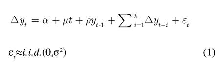
where ∆ represents first difference of the series, the term μ indicates a trend variable, and εt is the white noise term. ADF test is only valid under the assumption of i.i.d. processes. The null hypothesis implies that yt series contains a unit root when ρ=0. The rejection of the null hypothesis implies the stationarity of the series, implying that there is no unit root. The optimal lag length is determined by using the appropriate information criteria, such as Akaike information criterion (AIC) or the Schwarz information criterion (SIC).
PP test is a generalization of the Dickey-Fuller test and described as follows:
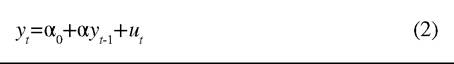
where ut is the white noise term. Philips and Perron (1988) modified the ADF test by allowing the error disturbances to be weakly dependent and heterogeneously distributed, since the ADF test assumes that errors are statistically independent and have constant variance. This test tends to be more robust to a wide range of serial correlations and time-dependent heteroscedasticity.
Unlike the ADF and PP unit root tests, KPSS assumes the stationarity of the series as the null hypothesis and the rejection of the null hypothesis indicates a non-stationary time series. The KPSS test uses a frequency zero spectrum estimation of the residuals in:

The KPSS test is one-sided Lagrange Multiplier (LM) test and is described as follow:
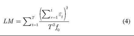
where f0 is the estimator of the residual spectrum at frequency zero.
Cointegrating Vectors
If two or more variables are cointegrated, there may exist stationary linear combinations of these variables. In absence of a cointegrating relationship among the variables, the variables have no long-run interdependence and can drift arbitrarily from each other (e.g. Engle & Granger, 1987; Johansen; 1988). Johansen’s methodology (Johansen, 1988; Johansen & Juselius; 1990) is applied to determine whether stock prices of developed and emerging markets move together over the long run.
Johansen cointegration approach, which takes its starting point in the vector autoregressive (VAR) analysis, utilizes maximum likelihood estimates to test for the number of cointegrating relationships in the multivariate system1. This approach relies on the relationship between the rank of a matrix and its characteristic roots (eigenvalues). Consider a VAR of order p:
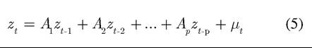
where zt is an n x 1 vector of variables, each of Ai represents a n x n matrix of parameters and μt is a zero mean white noise vector process. The VAR representation is also re-written as follows: 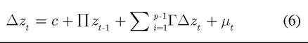
where
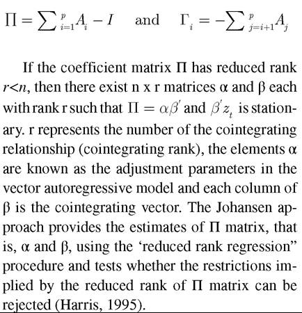
In order to determine the rank of matrix Π (that is, the number of cointegrating vectors), the characteristic roots or eigenvalues, λ of Π are estimated. Based on Johansen cointegration approach, two types of test statistics can be used for the hypothesis of the existence of r cointegrating vectors, maximum likelihood-based trace test (λ ) and maximum eigenvalue test (λ ), which are computed by using the following formulas:
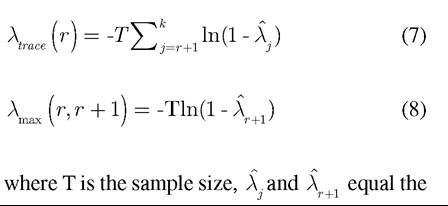
estimated values of the characteristic roots (eigenvalues) obtained from the Π matrix, r is the number of cointegrating vectors. The trace test evaluates the null hypothesis of the existence of at most r distinct cointegrating vectors against the alternative hypothesis of n cointegtaing vectors, whereas the maximum eigenvalue tests the null hypothesis of r cointegrating vectors against the alternative hypothesis of r+1 cointegrating vec-
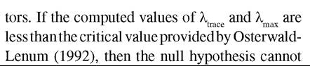
be rejected. The optimal lag structure of vector autoregression model is determined by using Akaike Information Criterion (AIC) and Schwarz Bayesian Criterion (SBC).
On the basis of Johansen approach, two alternative models were conducted to compare and contrast the linkages among the stock markets in the multivariate system; model 1, a model with no trend and model 2, a model with a linear trend in the cointegrating vector.
Error Correction and Granger Causality
The direction of the relationship between the variables was investigated by employing the causality test based on Granger’s approach (Granger, 1969). The linear Granger causality approach stated a testable definition of causality in terms of predictability in a set of non-cointegrated variables. In the presence of cointegration, standard Granger causality test is misspecified and a vector error correction model (VECM) can be formulated that captures both the long-run relationship and the short-run dynamics of the variables. The VECM depicts the feedback process and adjustment speed of short-run deviations towards the long-run equilibrium path. For two cointegrated series, xt and yt, the error correction mechanism can take the following forms: 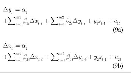
where y1 and y2 are the error correction terms. The magnitude of the coefficients of these error correction terms represents the speed of adjustment back to the long-run equilibrium after the market shock. In the case of large coefficients, reversion to the long-run equilibrium will be rapid and z will be highly stationary.
DATA
The dataset is comprised of the daily stock index closing prices from the sample markets from April 26, 2004 through March 8, 2013, obtained from Matriks Database. While the US, the UK and Germany were selected as representative for developed countries, the stock market indices of Brazil, Hungary, China, Taiwan, Poland and Turkey represented emerging stock markets (selected on the basis oftheir representativeness of emerging stock markets). Each stock price indices is denominated in US dollars. Any observations affected by national or other holidays are removed from the sample. Following the removal of these non trading days, 1991 observations were remained. As a means of conducting the impact of the global crisis on stock markets, the sample period was divided into two sub-periods. The beginning of August 2007 is chosen as the moment when the global financial crisis began to demonstrate its full manifestations on international stock markets. The first sub-period covers from April, 26 2004 to July, 31 2007. The second sub-period is from August, 1, 2007 to March, 8, 2013 corresponding to the post-crisis period.
The Lehman Brothers’ collapse in September 2008 is used by many researchers as the event which reflects the beginning of the crisis on international financial markets. However, a more thorough investigation demonstrates manifestations of the crisis in the second half of 2007, and spreading across economies, and engulfing developed and emerging economies, as shown in Figure 1.
The descriptive statistics of the return structure for the sample stock markets are represented in Table 1. The mean excess return is lower in the developed stock markets (SP500 and UKX) whereas the mean return is found to be higher for Brazil (BOVESPA) and Turkey (XU100). As anticipated, the emerging stock markets exhibit higher volatility, as indicated by larger standard deviation values with the exception of China, Taiwan and Poland. The results for skewness point to all stock indices being skewed to the left. The presence of high value of kurtosis for each index demonstrates leptokurtic distribution. The results for skewness and kurtosis statistics also signify the non-normality of returns, supported by Jarque- Bera statistics suggesting that any of the return series are not normally distributed.
The unconditional contemporaneous correlation matrix of the developed and emerging stock market indices providing important information for the subsequent Granger causality tests is reported in Table 2. Partitioning the period into two sub-periods, it is observed that there is an increase in the pairwise correlations among all developed and emerging stock markets, and all stock markets interconnections were strengthened after the crisis period, except those between Poland-Taiwan and Turkey-Taiwan. This result is accompanied by increases in the standard deviations of market returns and a reflection of the wider worldwide trend of greater global financial integration. The stock indices of the US, the UK and Germany indicate high and positive correlations, averaged between 80% and 95%, suggesting weak portfolio diversification benefits among the developed markets before and after the crisis period. The correlation coefficients report that developed markets are highly integrated with the emerging markets, namely Brazil, Poland, Hungary and Turkey, in the short run. These finding may be associated to closer economic ties, geographic proximity and EU union accession process. Surprisingly, the relatively isolated markets of China and Taiwan exhibit low correlations with the all
Figure 1. Stock markets (log) plots
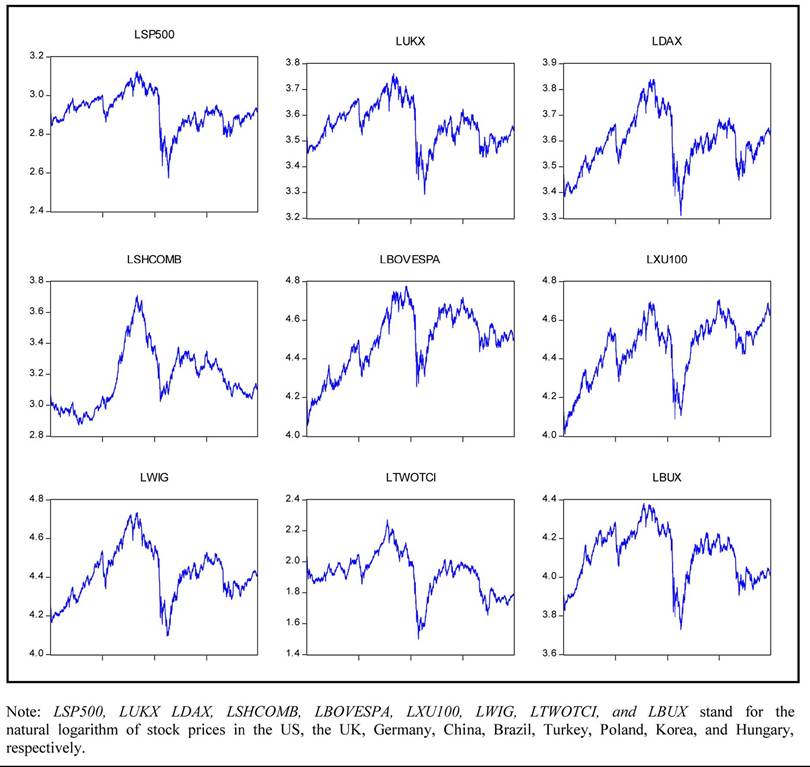
Table 1. Descriptive statistics
| Variables | Index | Mean | Std. Dev. | Max. | Min. | Kurt. | Skew. | JB |
| USA | SP500 | 0.000028 | 0.021537 | 0.163582 | -0.250623 | 19.92590 | -1.104741 | 24159.26 |
| UK | UKX | 0.000046 | 0.020292 | 0.141071 | -0.215918 | 15.56678 | -0.951582 | 13394.87 |
| Germany | DAX | 0.000202 | 0.021966 | 0.167980 | -0.230938 | 14.99537 | -0.753375 | 12119.02 |
| China | SHCOMB | 0.000047 | 0.021753 | 0.107980 | -0.166398 | 7.446637 | -0.467735 | 1712.037 |
| Brazil | BOVESPA | 0.000380 | 0.026484 | 0.187099 | -0.300137 | 17.12214 | -0.978196 | 16853.83 |
| Turkey | XU100 | 0.000626 | 0.025292 | 0.141483 | -0.259147 | 11.62690 | -0.840471 | 6405.232 |
| Poland | WIG | 0.000196 | 0.020806 | 0.107434 | -0.211730 | 12.61403 | -0.983965 | 7985.066 |
| Taiwan | TWOTCI | -0.000275 | 0.020134 | 0.098440 | -0.154339 | 9.076587 | -1.005101 | 3396.750 |
| Hungary | BUX | 0.000135 | 0.024268 | 0.152027 | -0.204375 | 11.80804 | -0.471713 | 6506.609 |
Note: Std. Dev. indicates standard deviation. Jarque-Bera (JB) normality test statistic has a chi-square distribution with 2 degrees of freedom.
Table 2. Unconditional correlation matrix
| Variables | SP500 | UKX | DAX | BOVESPA | BUX | SHCOMB | TWOTCI | WIG | XU100 | |
| Before Crisis | SP500 | 1.00000 | ||||||||
| UKX | 0.80992 | 1.00000 | ||||||||
| DAX | 0.79741 | 0.93994 | 1.00000 | |||||||
| BOVESPA | 0.81315 | 0.71708 | 0.69305 | 1.00000 | ||||||
| BUX | 0.58674 | 0.72372 | 0.68581 | 0.55849 | 1.00000 | |||||
| SHCOMB | 0.48699 | 0.48081 | 0.45204 | 0.46589 | 0.37862 | 1.00000 | ||||
| TWOTCI | 0.55105 | 0.61206 | 0.60165 | 0.47717 | 0.52212 | 0.41078 | 1.00000 | |||
| WIG | 0.70315 | 0.81717 | 0.77882 | 0.64361 | 0.79815 | 0.48646 | 0.61242 | 1.00000 | ||
| XU100 | 0.62375 | 0.73652 | 0.71054 | 0.58207 | 0.70175 | 0.42166 | 0.60282 | 0.73332 | 1.00000 | |
| After Crisis | SP500 | 1.00000 | ||||||||
| UKX | 0.83663 | 1.00000 | ||||||||
| DAX | 0.85376 | 0.93826 | 1.00000 | |||||||
| BOVESPA | 0.85513 | 0.82484 | 0.81753 | 1.00000 | ||||||
| BUX | 0.72547 | 0.79711 | 0.80002 | 0.72207 | 1.0000 | |||||
| SHCOMB | 0.48614 | 0.54682 | 0.53415 | 0.54745 | 0.49915 | 1.00000 | ||||
| TWOTCI | 0.56774 | 0.63697 | 0.61822 | 0.59737 | 0.56667 | 0.55563 | 1.00000 | |||
| WIG | 0.76539 | 0.85331 | 0.84827 | 0.76711 | 0.79856 | 0.54921 | 0.61561 | 1.00000 | ||
| XU100 | 0.72672 | 0.82083 | 0.80307 | 0.72768 | 0.73525 | 0.52871 | 0.61881 | 0.82251 | 1.00000 |
developed markets. Further investigation through cointegration techniques whether the short-term correlations among the developed and emerging markets support the existence of international diversification benefits for the long-term investment will be discussed in the next section.
EMPIRICAL RESULTS
Results of the Unit Root Test
To test for the presence of stochastic non-station- arity in the data, the integration order of the each stock index series is investigated using standard unit root tests. The ADF, PP and KPSS unit root tests are applied both with and without trend on the levels, and first differences of each series and the results are reported in Table 3. The null hypothesis of a unit root test is not rejected at the 1% significance level by both ADF and PP tests for any stock indices in the log levels. Hence, the first differences series reject the null hypothesis, indicating that they are integrated of order one, I (1). These findings are also supported by the KPSS test. The next step is to check whether the stock markets are cointegrated in the long-run.
Cointegration and Causality Analysis
Having established the unit root characteristics of the stock market indices, multivariate models can be conducted to allow examination of the presence or absence of cointegrating relationships among the emerging and developed markets. Johansen’s approach, which requires the estimation of VAR (p), is employed to analyze whether developed and emerging stock market indices are jointly integrated. The optimal number of lag (p) of the VAR is determined based on Akaike Information
Table 3. Unit root tests
| ADF | PP | KPSS | ||||||
| Level/First Difference | No Trend | Trend | No Trend | Trend | No Trend | Trend | ||
| Before Crisis | SP500 | Level | -0.912888 | -2.407005 | -0.964511 | -2.460582 | 2.175871* | 0.251923* |
| First Diff. | -26.78615* | -26.78068* | -26.77105 | -2676491 | 0.079112 | 0.048940 | ||
| UKX | Level | -0.894895 | -2.550933 | -0.885729 | -2.718559 | bgcolor=white>2.704174*0.306638* | ||
| First Diff. | -29.29536* | -29.28038* | -29.27603* | -29.26124* | 0.051895 | 0.047289 | ||
| DAX | Level | -0.044479 | -2.750244 | -0.029821 | -2.750244 | 3.000597* | 0.188509** | |
| First Diff. | -28.72627* | -28.74211* | -28.71673* | -28.73591* | 0.128175 | 0.056770 | ||
| BOVESPA | Level | -0.282233 | -2.718028 | -0.323188 | -2.809058 | 3.060504* | 0.159367** | |
| First Diff. | -27.16540* | -27.16174* | -27.15515* | -2.715515* | 0.069166 | 0.038772 | ||
| BUX | Level | -1.077205 | -1.985628 | -0.994449 | -2.003609 | 2.664819* | 0.559949* | |
| First Diff. | -17.86755* | -17.85637* | -26.28736* | -26.27153* | 0.068792 | 0.068611 | ||
| SHCOMB | Level | 2.605255 | -0.376504 | 2.532590 | -0.488841 | 2.151006* | 0.767245* | |
| First Diff. | -29.56490* | -30.10609* | -29.53252* | -30.12250* | 1.480166* | 0.043579 | ||
| TWOTCI | Level | 0.716924 | -2.127234 | 0.627430 | -2.345925 | 2.257821* | 0.320716* | |
| First Diff. | -25.26770* | -25.49099* | -25.29669* | -25.48461* | 0.598559** | 0.087796 | ||
| WIG | Level | 0.341360 | -3.226443*** | 0.229546 | -3.393609*** | 3.250448* | 0.210547** | |
| First Diff. | -18.03036* | -18.05672* | -27.84568* | -27.86570* | 0.129527 | 0.032317 | ||
| XU100 | Level | -0.903574 | -2.121018 | -0.799365 | -2.093131 | 2.779769* | 0.416620* | |
| First Diff. | -26.08118* | -26.06466* | -26.05255* | -26.03574* | 0.061412 | 0.064951 | ||
| After Crisis | SP500 | Level | -2.202141 | -2.023264 | -2.033968 | -1.803011 | 0.841325* | 0.536699* |
| First Diff. | -6.953302* | -7.008950* | -38.04734* | -38.07735* | 0.165527 | 0.055397 | ||
| UKX | Level | -2.216877 | -2.165856 | -2.170975 | -2.115511 | 1.103529* | 0.414235* | |
| First Diff. | -7.140590* | -7.166269* | -35.41577 | -35.41865 | 0.103598 | 0.047970 | ||
| DAX | Level | -2.166148 | -2.040914 | -2.143726 | -1.967271 | 0.839947* | 0.442236* | |
| First Diff. | -7.367854* | -7.401755* | -35.04438* | -35.05363* | 0.133411 | 0.052715 | ||
| BOVESPA | Level | -2.255436 | -2.485370 | -1.999167 | -2.224254 | 0.706801** | 0.260344* | |
| First Diff. | -6.671278* | -6.670470* | -35.51938* | -35.50367* | 0.056757 | 0.056087 | ||
| BUX | Level | -2.183812 | -2.255926 | -2.047045 | -1.964740 | 1.100577* | 0.330741* | |
| First Diff. | -6.542570* | -6.552310* | -32.38393* | -32.39456* | 0.119021 | 0.083896 | ||
| SHCOMB | Level | -1.621405 | -1.760921 | -1.538913 | -1.719635 | 2.462739* | 0.347828* | |
| First Diff. | -32.09488* | -32.09187* | -32.09564* | -32.09257* | 0.110324 | 0.079123 | ||
| TWOTCi | Level | -2.117293 | -2.074556 | -2.270862 | -1.957332 | 1.184502* | 0.340903* | |
| First Diff. | -6.780843 | -6.807140 | -29.04153 | -29.08944 | 0.239533 | 0.139857*** | ||
| WIG | Level | -2.085591 | -1.884309 | -2.171979 | -1.872130 | 0.880924* | 0.425195* | |
| First Diff. | -10.56787* | -10.60466* | -31.58764* | -31.65005* | 0.216596 | 0.091486 | ||
| Level | -1.934897 | -2.177374 | -1.480473 | -1.833652 | 0.801141* | 0.345696* | ||
| First Diff. | -6.592990* | -6.614105* | -32.99722* | -33.00757* | 0.164509 | 0.084370 | ||
Note: SP500, UKX, DAX, BOVESPA, BUX, SHCOMB, TWOTCI, WIG and XU100 represent natural logarithm of stock price index.
ADF: Optimum lag is selected according to the AIC, critical values are based on MacKinnon (1991); critical values are -3.43 (99%), -2.86 (95%), -2.56 (90%) and -3.96 (99%), -3.41 (95%), -3.13 (90%) with no trend and with trend, respectively. PP: Optimum lag is selected according to the AIC, critical values are based on MacKinnon (1991); critical values are -3.43 (99%), -2.86 (95%), -2.56 (90%) and -3.96 (99%), -3.41 (95%), -3.13 (90%) with no trend and with trend, respectively. KPSS: Optimum lag is selected according to Schwert (1989); critical values are 0.216, 0.146, and 0.119 for the model with trend; 0.739, 0.463, 0.347 for the model without trend and for 1, 5, and 10% respectively (KPSS, 1992).
*, ** and *** denote rejection of null hypothesis at 1, 5 and 10%, respectively
Criterion (AIC). The determination of the order of the stock market indices in the VAR model depends upon the market capitalization value of each series. As mentioned above, two alternative models, a model without trend (model 1) and a model with a linear trend in the cointegrating equation (model 2), are employed to compare whether the inclusion of trend in the cointegrating vector alters the critical values of the test statistics. Table 4 and Table 5 present the results of the λ and λ tests, respectively. In the case of λtace test, the empirical findings of both models indicate that there are at most two cointegrating vectors for the pre- and post-crisis period, since H0 of r≤2 is not rejected at the 5% significance level. The presence of a long run relationship is an evidence of financial integration among these markets, which will accelerate the adjustment process from the short run to the long run. However, the empirical findings of λ test reveal the max
presence of one cointegrating vector only for the post-crisis period in both versions of the model. Since the tests for cointegration utilizing both the λ and λ statistics represent different results, λ test is more preferable than λ test (Johansen & Juselius, 1990)2.
Since cointegration tests carried out for the developed and emerging stock markets show a long run relationship, the coefficients in the cointegrating vector inform us the extent of the stock
Table 4. Tests for the presence of cointegrating vectors
| Null | Eigenvalues | Critical Values at 95% | |||
| Model 1 | Model 2 | Model 1 | Model 2 | ||
| Before Crisis | r=0 | 0.066967 | 0.073483 | 197.3709 | 228.2979 |
| r≤1 | 0.058310 | 0.058320 | 159.5297 | 187.4701 | |
| r≤2 | 0.048784 | 0.048821 | 125.6154 | 150.5585 | |
| r≤3 | 0.035751 | 0.040572 | 95.75366 | 117.7082 | |
| r≤4 | 0.029238 | 0.034702 | 69.81889 | 88.80380 | |
| r≤5 | 0.020225 | 0.028011 | 47.85613 | 63.87610 | |
| r≤6 | 0.012821 | 0.019247 | 29.79707 | 42.91525 | |
| r≤7 | 0.006984 | 0.010552 | 15.49471 | 25.87211 | |
| r≤8 | 0.000100 | 0.005252 | 3.841466 | 12.51798 | |
| After Crisis | r=0 | 0.049245 | 0.058079 | 197.3709 | 228.2979 |
| r≤1 | 0.036437 | 0.036719 | 159.5297 | 187.4701 | |
| r≤2 | 0.029414 | 0.032977 | 125.6154 | 150.5585 | |
| r≤3 | 0.024117 | 0.029395 | 95.75366 | 117.7082 | |
| r≤4 | 0.015519 | 0.018378 | 69.81889 | 88.80380 | |
| r≤5 | 0.013235 | 0.013546 | 47.85613 | 63.87610 | |
| r≤6 | 0.008345 | 0.013020 | 29.79707 | 42.91525 | |
| r≤7 | 0.005440 | 0.008332 | 15.49471 | 25.87211 | |
| r≤8 | 0.000335 | 0.005422 | 3.841466 | 12.51798 | |
Table 5. Tests for the number of cointegrating vectors
| Null | Test | Critical Values at 95% | |||
| Model 1 | Model 2 | Model 1 | Model 2 | ||
| Before Crisis | r=0 | 53.71892 | 59.15063 | 58.43354 | 62.75215 |
| r=1 | 46.56136 | 46.56956 | 52.36261 | 56.70519 | |
| r=2 | 38.76086 | 38.79100 | 46.23142 | 50.59985 | |
| r=3 | 28.21457 | 32.09882 | 40.07757 | 44.49720 | |
| r=4 | 22.99769 | 27.37151 | 33.87687 | 38.33101 | |
| r=5 | 15.83479 | 22.01867 | 27.58434 | 32.11832 | |
| r=6 | 10.00041 | 15.06163 | bgcolor=white>21.1316225.82321 | ||
| r=7 | 5.431379 | 8.221358 | 14.26460 | 19.38704 | |
| r=8 | 0.077887 | 4.081154 | 3.841466 | 12.51798 | |
| After Crisis | r=0 | 61.05371* | 72.33945* | 58.43354 | 62.75215 |
| r=1 | 44.87433 | 45.22830 | 52.36261 | 56.70519 | |
| r=2 | 36.09549 | 40.54127 | 46.23142 | 50.59985 | |
| r=3 | 29.51455 | 36.07129 | 40.07757 | 44.49720 | |
| r=4 | 18.91000 | 22.42549 | 33.87687 | 38.33101 | |
| r=5 | 16.10795 | 16.48920 | 27.58434 | 32.11832 | |
| r=6 | 10.13128 | 15.84435 | 21.13162 | 25.82321 | |
| r=7 | 6.595037 | 10.11552 | 14.26460 | 19.38704 | |
| r=8 | 0.405462 | 6.573618 | 3.841466 | 12.51798 | |
Notes: H1(r) against H1(n).
Model 1: Model without trend.
Model 2: Model with a linear trend in the cointegrating equation; critical values from Ostenwald-Lenum (1992).
Notes: H1(r) against H1(r + 1).
Model 1: Model without trend.
Model 2: Model with a linear trend in the cointegrating equation; critical values from Ostenwald-Lenum (1992).
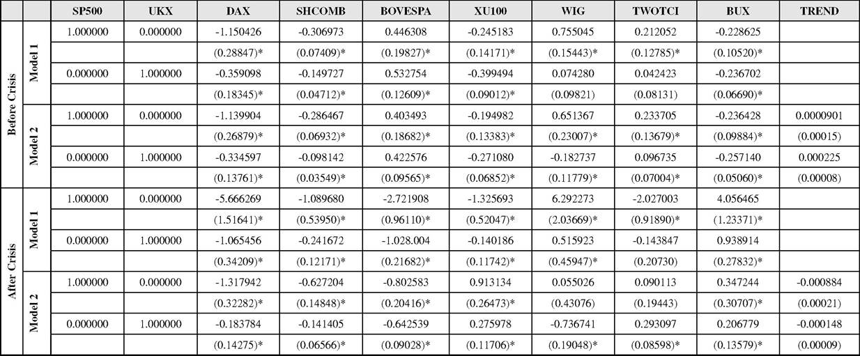
market integration in the long run. With respect to the reported two cointegrated vectors according to the λ test, the influence of two developed markets (the US and the UK) on emerging equity markets was investigated. Table 6 reports the normalized cointegration vector from the two versions of the model for the pre- and post-crisis period. The relative size of the coefficient of the cointegrating vector provides considerable information about the role of the individual stock markets in the group.
The empirical findings of model 1 and model 2 indicate that the US stock market has a positive long run impact on Brazil, Poland and Taiwan, whereas a negative long run impact on Germany, China, Turkey and Hungary in the pre-crisis period. In the post-crisis period, the direction of the relationship between developed (the US) and emerging markets remains the same, except for Brazil in model 1, and Brazil and Turkey in model 2. Surprisingly, the prevailing significant relationship disappears between the US and two emerging markets, namely Poland and Taiwan, in model 2. The results indicate that these two pair-wise countries have relatively less financial importance in comparison with the other emerging countries in our sample. As noted by Forbes and Chinn, 2004, after the divergence of economic and industrial structures of countries, the degree of financial integration between the stock markets may also differ. Given the primary role of the US, the UK and Germany, in terms of trading volume, market capitalization, depth and liquidity, these findings are reasonable and consistent with the results of previous studies (Ratanapakorn & Sharma, 2002; Syriopoulos, 2006, 2007 and 2011). Overall, the findings reveal that the global crisis results both in changes in the direction of the long-run relationship among some markets, and causes striking increases in the relative size of the coefficients of all markets in the cointegrating vector. The increase in the magnitude of the interrelationship and dynamic linkages has in the post-crisis period among the developed and emerging markets is due to the herding behavior of the investors throughout the financial crisis period, and growing inflow and outflow of portfolio investments across developed and emerging markets.
The co-movements and linkages among these stock markets may be attributed to international financial globalization, and integration as well as, to the common path of their economies. The global crisis, as an external shock to the domestic markets, affected all emerging markets, leading to a long-run equilibrium path. Therefore, the presence of cointegrating relationship between developed and emerging markets reveals that the latter have become increasingly integrated with the former after crisis period, implying that long- run international investors who seek to diversify their portfolios across the emerging and developed markets should expect only modest long-term portfolio benefits. These findings are in line with the previous empirical findings (Meric et al., 2012). From such an investment allocation, it has become more difficult to reduce the portfolio risk because the diversification benefit is less effective across the cointegrated stock markets.
Error Correction and Causality
In the presence of cointegrating vectors across the developed and emerging markets under study, the possible short-run (uni-or bi-directional) Granger causal relationship among the stock markets is investigated through the VECM estimations. In addition to the short run causalities, the VECM captures both speed of adjustment through the long-run equilibrium path and lead-lag relationships between developed and emerging markets. Hence, it is possible to draw conclusions from these results for the international investment allocation.
In the VEC model, there are two approaches to estimating the causal relationship between the stock markets; one is through the error correction term, which estimates the response of the dependent variable to departure from equilibrium and
Table 6. Nonnalized Cointegrated vector
Notes: Figures in () are standard errors.
Model 1: Model without trend.
Model 2: Model with a linear trend in the cointegrating equation. * indicates 1% significant level.
Uonal Portfolio Diversification Benefits among Developed and Emerging Markets
1315
the other one is through the lagged differences of variables. The results of Granger causality tests through VECM between the stock markets are reported in Tables 7 and 8. The optimal lag length for the VECM is selected based on the Akaike Information Criterion (AIC) for each sub-period.
In order to investigate the speed of adjustment to restoring long-run equilibrium in the dynamic model, the error correction terms are estimated, and the results are reported in Tables 7 and 8, Panel A. In the pre-crisis period, the ECT is found to be statistically insignificant in all developed markets except for the UK. In the post-crisis period, however, the UK ECT coefficient turned out to be insignificant. This may be explained by the fact that these developed markets appear statistically exogenous to the system and they determine the trends/paths that the other emerging markets will follow in the long-run, which is in line with the previous studies (Syriopoulos, 2007, 2011). For the
Table 7. VECM estimated for before crisis period
| Panel A. Error Correction Term Estimates | |||||||||||
| Variables | SP500 | UKX | DAX | bgcolor=white>SHCOMBBOVESPA | XU100 | WIG | TWOTCI | BUX | |||
| ECT | 0.019227 | 0.028382** | 0.022253 | 0.007154 | 0.052440* | 0.002008 | -0.016508 | -0.035720** | -0.021450 | ||
| (0.01246) | (0.01269) | (0.01448) | (0.01926) | (0.02043) | (0.02117) | (0.01616) | (0.01567) | (0.01726) | |||
| [ 1.54313] | [ 2.23663] | [ 1.53667] | [ 0.37150] | [ 2.56709] | [ 0.09487] | [-1.02125] | [-2.27941] | [-1.24296] | |||
| Panel B. Granger Causality Test | |||||||||||
| F Statistic | F Statistic | ||||||||||
| SP500→UKX | 25.5556* | BOVESPA→XU100 | 26.6222* | ||||||||
| SP500→DAX | 21.7645* | BOVESPA→WIG | 18.5774* | ||||||||
| SP500→SHCOMB | 3.20090** | BOVESPA→TWOTCI | 13.2294* | ||||||||
| SP500→BOVESPA | 0.44459 | BOVESPA→BUX | 21.5436* | ||||||||
| SP500→XU100 | 23.7682* | XU100→SP500 | 0.37008 | ||||||||
| SP500→WIG | 13.9952* | XU100→UKX | 2.96367*** | ||||||||
| SP500→TWOTCI | 11.5537* | XU100→DAX | 0.41666 | ||||||||
| SP500→BUX | 13.2930* | XU100→SHCOMB | 3.48315** | ||||||||
| UKX→SP500 | 0.62927 | XU100→BOVESPA | 0.37259 | ||||||||
| UKX→DAX | 0.44849 | XU100→WIG | 0.54658 | ||||||||
| UKX→SHCOMB | 2.51235*** | XU100→TWOTCI | 2.70534*** | ||||||||
| UKX→BOVESPA | 0.93512 | XU100→BUX | 0.39053 | ||||||||
| UKX→XU100 | 2.52575*** | WIG→SP500 | 2.82542*** | ||||||||
| UKX→WIG | 0.25023 | WIG→UKX | 0.74780 | ||||||||
| UKX→TWOTCI | 4.85384* | WIG→DAX | 1.88422 | ||||||||
| UKX→BUX | 1.61886 | WIG→SHCOMB | 3.75743** | ||||||||
| DAX→SP500 | 1.19981 | WIG→BOVESPA | 4.92078* | ||||||||
| DAX→UKX | 0.83568 | WIG→XU100 | 0.80587 | ||||||||
| DAX→SHCOMB | 3.10944** | WIG→TWOTCI | 7.88343* | ||||||||
| DAX→BOVESPA | 2.63092*** | WIG→BUX | 0.38887 | ||||||||
| DAX→XU100 | 3.62695** | TWOTCI→SP500 | 0.73428 | ||||||||
Table 7. Continued
| DAX→WIG | 0.45320 | TWOTCI→UKX | 1.27798 |
| DAX→TWOTCI | 7.31959* | TWOTCI→DAX | 2.43938*** |
| DAX→BUX | 1.49686 | TWOTCI→SHCOMB | 2.02329 |
| SHCOMB→SP500 | 3.35566** | TWOTCI→BOVESPA | 0.56392 |
| SHCOMB→UKX | 0.52000 | TWOTCI→XU100 | 1.91855 |
| SHCOMB→DAX | 0.36999 | TWOTCI→WIG | 2.16633 |
| SHCOMB→BOVESPA | 4.30560** | TWOTCI→BUX | 0.00516 |
| SHCOMB→XU100 | 0.79256 | BUX→SP500 | 0.51066 |
| SHCOMB→WIG | 1.26152 | BUX→UKX | 1.26181 |
| SHCOMB→TWOTCI | 2.17713 | BUX→DAX | 0.04942 |
| SHCOMB→BUX | 0.62341 | BUX→SHCOMB | 3.28051** |
| BOVESPA→SP500 | 0.86576 | BUX→XU100 | 0.87568 |
| BOVESPA→UKX | 20.5822* | BUX→BOVESPA | 0.22040 |
| BOVESPA→DAX | 13.4738* | BUX→WIG | 0.88558 |
| BOVESPA→SHCOMB | 6.43574* | BUX→TWOTCI | 3.11197** |
Notes: Figures in (), [ ] are standard errors and t-statistics, respectively. *,**,*** indicate 1%, 5% and 10% significant level, respectively.
Table 8. VECM estimated for after crisis period
| Panel A. Error Correction Term Estimates | |||||||||||
| Variables | SP500 | UKX | DAX | SHCOMB | BOVESPA | XU100 | WIG | TWOTCI | BUX | ||
| ECT | -0.000805 | 0.004990 | 0.003542 | -0.001695 | 0.001856 | 0.000769 | -0.008811** | -0.000449 | -0.008218*** | ||
| (0.00437) | (0.00395) | (0.00429) | (0.00389) | (0.00501) | (0.00458) | (0.00387) | (0.00372) | (0.00458) | |||
| [-0.18399] | [ 1.26242] | [ 0.82517] | [-0.43579] | [ 0.37008] | [ 0.16774] | [-2.27685] | [-0.12058] | [-1.79480] | |||
| Panel B. Granger Causality test | |||||||||||
| F Statistic | F Statistic | ||||||||||
| SP500→UKX | 18.1776* | BOVESPA→XU100 | 2.10407*** | ||||||||
| SP500→DAX | 10.1389* | BOVESPA→WIG | 0.41388 | ||||||||
| SP500→SHCOMB | 10.2290* | BOVESPA→TWOTCI | 4.99398* | ||||||||
| SP500→BOVESPA | 6.35331* | BOVESPA→BUX | 4.73304* | ||||||||
| SP500→XU100 | 5.74039* | XU100→SP500 | 2.04324 | ||||||||
| SP500→WIG | 3.51748** | XU100→UKX | 1.81410 | ||||||||
| SP500→TWOTCI | 7.71023* | XU100→DAX | 1.49023 | ||||||||
| SP500→BUX | 8.65956* | XU100→SHCOMB | 7.84621* | ||||||||
| UKX→SP500 | 2.6.316** | XU100→BOVESPA | 1.65225 | ||||||||
| UKX→DAX | 0.18178 | XU100→WIG | 1.53655 | ||||||||
| UKX→SHCOMB | 11.5630* | XU100→TWOTCI | 4.33206* | ||||||||
| UKX→BOVESPA | 2.46581*** | XU100→BUX | 5.39618* | ||||||||
| UKX→XU100 | 2.05937 | WIG→SP500 | 5.26514* | ||||||||
Table 8. Continued
| UKX→WIG | 2.75126** | WIG→UKX | 6.51636* |
| UKX→TWOTCI | 4.27446* | WIG→DAX | 6.29729* |
| UKX→BUX | 2.00898 | WIG→SHCOMB | 10.6575* |
| DAX→SP500 | 1.15596 | WIG→BOVESPA | 4.57119* |
| DAX→UKX | 0.06568 | WIG→XU100 | 2.07568 |
| DAX→SHCOMB | 8.51174* | WIG→TWOTCI | 6.42116* |
| DAX→BOVESPA | 1.80968 | WIG→BUX | 7.42057* |
| DAX→XU100 | 1.64853 | TWOTCI→SP500 | 3.10044** |
| DAX→WIG | 2.15398*** | TWOTCI→UKX | 4.27735* |
| DAX→TWOTCI | 5.02095* | TWOTCI→DAX | 2.74514** |
| DAX→BUX | 1.43772 | TWOTCI→SHCOMB | 4.33019* |
| SHCOMB→SP500 | 1.33218 | TWOTCI→BOVESPA | 5.83655* |
| SHCOMB→UKX | 1.60980 | TWOTCI→XU100 | 0.70372 |
| SHCOMB→DAX | 0.69820 | TWOTCI→WIG | 3.84063* |
| SHCOMB→BOVESPA | 3.75617** | TWOTCI→BUX | 1.04021* |
| SHCOMB→XU100 | 0.20826 | BUX→SP500 | 0.50687 |
| SHCOMB→WIG | 1.49505 | BUX→UKX | 1.17614 |
| SHCOMB→TWOTCI | 0.54385 | BUX→DAX | 0.50896 |
| SHCOMB→BUX | 2.60136** | BUX→SHCOMB | 5.71579* |
| BOVESPA→SP500 | 0.58076 | BUX→BOVESPA | 0.42239 |
| BOVESPA→UKX | 3.51280** | BUX→XU100 | 0.94132 |
| BOVESPA→DAX | 0.87162 | BUX→WIG | 1.11205 |
| BOVESPA→SHCOMB | 8.25508* | BUX→TWOTCI | 2.50297*** |
Notes: Figures in (), [ ] are standard errors and t-statistics, respectively. *,**,*** indicate 1%, 5% and 10% significant level, respectively.
emerging markets, ECT is found to be statistically significant for Brazil and Taiwan pre-crisis period, whereas the post-crisis coefficient estimates for the ECT are found to be statistically significant mainly in cases of Poland and Hungary. These results imply that these emerging markets seem to be potentially influenced by short-run shocks in the developed markets. The larger ECT coefficients for Brazil stock market before the crisis period and Poland and Hungary stock markets after the crisis period state that a deviation from the long-run equilibrium following a short-run shock is adjusted more rapidly compared to the other stock markets. This may be linked to the fact that these emerging markets, namely Brazil, Poland and Hungary, are more closely integrated with the developed markets.
The results of the direction of the causal relationship and lead-lag effects between each pair of markets in our dataset for the two sub-periods are summarized in Tables 7 and 8, Panel B. The empirical results from the causality test support the international leading role of the US and German markets, implying that these markets have a strong impact on all other stock markets in both sub-periods, which is consistent with the previous studies (Massih & Massih, 1997; Ratanapakorn & Sharma, 2002). These findings appear to be reasonable because of their market capitalization as well as foreign direct capital inflows and investors’ stock investments in the emerging markets (Hanousek & Filer, 2000). Of all the emerging markets under study, the one that seems to have the most influence of the US market is China, due to the geographic proximity, robust trade and financial transactions and the highest market capitalization. As expected, the pre-crisis causal relationship between the US and China is found to be bi-directional, while Chinese stock market is not seen to exert any significant impact on the other developed countries, Germany and the UK. The global financial crisis that started in the US caused a slowdown of the growth in China. Hence, after the crisis period, the influence of China on the US stock market has totally disappeared. As a consequence, the recent worldwide financial crisis has proved that Chinese stock market remains isolated from the external shocks which originating from developed stock markets, especially, the US.
Surprisingly, for the pair-wise setting, only Poland and Taiwan represent bi-directional causal relationship among the developed and emerging markets after the crisis period, as in the case of unilateral causal effects of Poland on the US, China and Brazil; and Taiwan on Germany. During this recent crisis, the contagion originating in the US spread quickly to the other countries around the world. The episodic evidence of results confirms the possible short-run granger causal relationship among the stock markets post-crisis. On the other hand, taking the results of the tests for the Hungarian stock market into consideration, it seems that there was no change in the nature of the causal relationship over the time period. It is worth pointing out that no causal bi-directional relationship is detected between the US and Brazil for either sub-periods, despite the strength of trade, the geographical proximity, cultural factors and portfolio fund flows between the two economics. In the pair-wise setting of Turkey and the UK, it is noted that the initial evidence of causal relationship disappears in the post-crisis.
FUTURE RESEARCH DIRECTIONS
The dynamic co-movements and causal relationship among the developed and emerging markets under study studied in this chapter provides a guide for future research. In order to further understand the stock market interdependencies, in addition to conventional cointegration tests, regime-shifting cointegration models will be studied since they allow structural changes in the cointegrating vectors. Moreover, future research at these nodes will include variance decomposition and impulse response analysis. Variance decomposition analysis, which provides a quantitative measure of the linkages among the stock markets, explains the degree of a movement in a stock market through other markets, in regard to the percentage of forecast error variance of that market. Impulse response analysis, as a further investigation of the short-term relationship among stock markets, maps out the responsiveness of a particular stock market to the shocks emerging from other stock markets, and examines whether the impact of an unexpected shock is permanent or transitory in each stock market.
Additionally, future research at these nodes will capture the impact of the recent global crisis on the time-varying correlation dynamics by employing GARCH models. If stock returns exhibit GARCH effects, it is reasonable to expect that the cointegrating relationship among markets could be affected by the presence of time-varying volatility. Hence, the future research adopts the modified cointegration tests with time-varying volatility effects.
CONCLUSION
This chapter investigates short and long-run dynamic linkages and causal effects among stock markets of developed countries, particularly the US, the UK and Germany, and emerging countries namely Brazil, Poland, Hungary, Taiwan, China and Turkey over the period 2004-2013, and examines whether the developed and emerging stock markets have been affected by the recent global financial crisis. The time period is considered long enough for stock markets to show the effects of the global crisis; therefore, the empirical findings have direct implications for the assessment of risk and return characteristics and will be helpful in understanding the short and long-run diversification benefits for international investors.
The multivariate cointegration test results demonstrate that the global crisis changes the direction of the long-run relationship between the US-Brazil, the US-Hungary, the UK-Brazil and the UK-Hungary stock market pairs for two alternative models. However, only, the integration of the US and the UK with Turkey becomes positive for one of the cointegration model after the crisis period although it is negative before the crisis period. The magnitude of the coefficients of the cointegrating vector increases after the crisis period among the developed and emerging markets which is informative on the respective role of the each market. The presence of high degree of correlations across emerging and developed countries can be attributed to an increase in economic and financial integration among these countries, and in fact, there is a growing inflow and outflow of portfolio investments across developed and emerging markets, which is a result of herding behavior of investors throughout the crisis period. The results of the Granger causality tests clearly reveal that the interdependencies among stock markets are generally greater in the post-crisis period. The US stock market has the greatest impact on all emerging markets in either sub-period, supporting the leading influential role of the US.
As expected, all empirical analyses confirm the strong interrelations between the stock markets after the crisis period, which, in turn, implies that the benefits of international portfolio diversification disappear after financial turmoil. These findings indicate that investors who try to diversify their portfolios among emerging markets as well as developed countries may expect rather short-run portfolio gains, since investment risk cannot be reduced, and market shocks can affect the portfolio returns. These results are in line with the findings of Grubel and Fadner (1971), Ripley (1973), and Panton et al. (1976) who point out that the benefits from international diversification will be reduced in the long run, because long-run interrelationship between stock markets are higher than those in the short run.
REFERENCES
Arshanapalli, B., & Doukas, J. (1993). International stock market linkages: Evidence from pre- and post-October 1987 period. Journal of Banking & Finance, 17(1), 193-208. doi:10.1016/0378- 4266(93)90088-U
Bessler, D. A., & Yang, J. (2003). The structure of interdependence in international stock markets. Journal OfInternational Money and Finance, 22, 261-287. doi:10.1016/S0261-5606(02)00076-1
Cheung, Y., & Lai, K. (1993). Finite-sample sizes of Johansen’s likelihood ratio tests for cointegration. Oxford Bulletin of Economics and Statistics, 55, 313-328. doi:10.1111/j.1468-0084.1993. mp55003003.x
Coeurdacier, N., & Guibaud, S. (2011). International portfolio diversification is better than you think. Journal of International Money and Finance, 30, 289-308. doi:10.1016/j.jimon- fin.2010.10.003
Corhay, A., Rad, A. T., & Urbain, J. P. (1993). Common stochastic trends in European stock markets. Economics Letters, 42, 385-390. doi:10.1016/0165-1765(93)90090-Y
Corhay, A., Rad, A. T., & Urbain, J. P. (1995). Long run behavior of Pacific-Basin stock prices. Applied Financial Economics, 5, 11-18. doi:10.1080/758527666
Demian, C.-V. (2011). Cointegration in Central and East European markets in light of EU accession. Journal OfInternational Financial Markets, Institutions and Money, 21, 144-155. doi:10.1016/j. intfin.2010.10.002
Dickey, D. A., & Fuller, W. A. (1979). Distribution of the estimators for autoregressive time series with a unit root. Journal of the American Statistical Association, 74(366), 427-431. doi:10.2307/2286348
Dickey, D. A., & Fuller, W. A. (1981). Likelihood ratio statistics for autoregressive time series with a unit root. Econometrica, 49(4), 1057-1072. doi:10.2307/1912517
Dickinson, D. G. (2000). Stock market integration and macroeconomic fundamentals: An empirical analysis. Applied Financial Economics, 10, 261-276. doi:10.1080/096031000331671
Eiteman, D. K., Stonehill, A. I., & Moffett, M.
H. (2010). Multinational businessfinance. Upper Saddle River, NJ: Pearson.
Elton, E. J., & Gruber, M. J. (1995). Modern portfolio theory and investment analysis. New York: J. Wiley and Sons.
Engle, R. F., & Granger, C. W. J. (1987). Cointegration and error correction: Representation, estimation, and testing. Econometrica, 55(2), 251-276. doi:10.2307/1913236
Fama, E. F., & MacBeth, J. D. (1973). Risk, return, and equilibrium: Empirical tests. The Journal of Political Economy, 81(3), 607-636. doi:10.1086/260061
Fan, W. (2001). An empirical study of co-integra- tion and causality in the Asia-Pacific stock market (Working Paper). New Haven, CT: Yale University.
Farrell, J. L. Jr. (1997). Portfolio management: Theory and application. New York: McGraw-Hill.
Forbes, K., & Chinn, M. (2004). A decomposition of global linkages in financial markets over time. The Review of Economics and Statistics, 86(3), 705-722. doi:10.1162/0034653041811743
Granger, C. W. J. (1969). Investigating causal relations by econometric models and cross- spectral methods. Econometrica, 37(3), 424-438. doi:10.2307/1912791
Grubel, H., & Fadner, K. (1971). The interdependence of international equity markets. The Journal of Finance, 26, 89-94. doi:10.1111/j.1540-6261.1971.tb00591.x
Gupta, R., & Guidi, F. (2012). Co-integration relationship and time varying co-movements among Indian and Asian developed stock markets. International Review of Financial Analysis, 21, 10-22. doi:10.1016/j.irfa.2011.09.001
Hanousek, K., & Filer, R. K. (2000). The relationship between economic factors and equity markets in Central Europe. Economics of Transition, 8, 99-126. doi:10.1111/1468-0351.00058
Haroon, H., Yasir, H. R., Azeem, S. S. W., & Ahmed, F. (2012). International portfolio diversification in developing equity markets of South Asia. Studies in Business and Economics, 7(1), 80-100.
Harris, R. (1995). Using cointegration analysis in econometric modelling. London: Prentice Hall, Harvester Wheatsheaf.
Hassan, M. K., & Naka, A. (1996). Short-run and long-run dynamic linkages among international stock markets. International Review of Economics & Finance, 5(4), 387-405. doi:10.1016/S1059- 0560(96)90025-8
Huang, B. N., Yang, C. W., & Hu, J. W. S. (2000). Causality and co-integration of stock markets among the United States, Japan and the South China growth triangle. International Review of Financial Analysis, 9(3), 281-297. doi:10.1016/ S1057-5219(00)00031-4
Hung, B. W. S., & Cheung, Y. L. (1995). Interdependence of Asian emerging equity markets. Journal of Business Finance & Accounting, 22(2), 281-288. doi:10.1111/j.1468-5957.1995. tb00684.x
Hwang, J. K. (2012). Dynamic correlation analysis of Asian stock markets. International Advances in
Economic Research, 18, 227-237. doi:10.1007/ s11294-012-9343-6
Janakiramanan, S., & Lamba, A. S. (1998). An empirical examination of linkages between Pacific-Basin stock markets. Journal of International Financial Markets, Institutions and Money, 8, 155-173. doi:10.1016/S1042-4431(98)00029-8
Johansen, S. (1988). Statistical analysis of cointegration vectors. Journal of Economic Dynamics & Control, 12(2), 231-254. doi:10.1016/0165- 1889(88)90041-3
Johansen, S., & Juselius, K. (1990). Maximum likelihood estimation and inference on cointegration -With applications to the demand for money. Oxford Bulletin of Economics and Statistics, 52, 169-210. doi:10.1111/j.1468-0084.1990. mp52002003.x
Karim, B. A., Majid, M. S. A., & Karim, S. A. (2009). Integration of stock markets between Indonesia and its major trading partners. Gadjah Mada International Journal of Business, 11(2), 229-252.
Kasa, K. (1992). Common stochastic trends in international stock markets. Journal of Monetary Economics, 29, 95-124. doi:10.1016/0304- 3932(92)90025-W
Kenourgios, D., & Samitas, A. (2011). Equity market integration in emerging Balkan markets. Research in International Business and Finance, 25, 296-307. doi:10.1016/j.ribaf.2011.02.004
Kwiatkowski, D., Phillips, P. C. B., Schmidt, P., & Shin, Y. (1992). Testing the null hypothesis of stationarity against the alternative of a unit root. Journal of Econometrics, 54, 159-178. doi:10.1016/0304-4076(92)90104-Y
Lau, S., & McInish, T. (1993). Co-movements of international equity returns: Comparison of the pre-and post-October 19, 1987, periods. Global Finance Journal, 4(1), 1-19. doi:10.1016/1044- 0283(93)90010-V
Lee, S., & Kim, S. (1993). Does the October 1987 crash strengthen the co-movements among national stock markets? Review of Financial Economics, 3(1), 89-102.
MacKinnon, J. G. (1991). Critical values for cointegration tests. In Long-run economic relationships: Readings in cointegration. Oxford, UK: Oxford University Press.
Malliaris, A. G., & Urrutia, J. L. (1992). The international crash of October 1987: Causality tests. Journal of Financial and Quantitative Analysis, 27(3), 353-364. doi:10.2307/2331324
Markowitz, H. (1952). Portfolio selection. The Journal of Finance, 7(1), 77-91.
Meric, G., Leal, R., Ratner, M., & Meric, I. (2001). Co-movements ofUS and Latin American equity markets before and after the 1987 crash. International Review of Financial Analysis, 10(3), 219-235. doi:10.1016/S1057-5219(01)00053-9 Meric, G., Lentz, C., Smeltz, W., & Meric, I. (2012). International evidence on market linkages after the 2008 stock market crash. The International Journal ofBusiness and Finance Research, 6(4), 45-58.
Niklewski, J., & Rodgers, T. (2012). Did the impact of the 2007financial crisis on market correlations reduce the benefits of international portfolio diversification? Economics, Finance and Accounting, Applied Research Working Paper Series.
Osterwald-Lenum, M. (1992). A note with quartiles as the asymptotic distribution of the maximum likelihood cointegration rank test statistics. Oxford Bulletin of Economics and Statistics, 54(3), 461-472. doi:10.1111/j.1468-0084.1992. tb00013.x
Pagano, M. (1993). Financial markets and growth: An overview. European Economic Review, 37, 613-622. doi:10.1016/0014-2921(93)90051-B
Panton, D., Lessig, I., & Joy, M. (1976). Comovement of international equity markets: A taxonomic approach. Journal of Financial and Quantitative Analysis, 11, 415-432. doi:10.2307/2330417
Phillips, P. C. B., & Perron, P. (1988). Testing for a unit root in time series regression. Biometrika, 75, 335-346. doi:10.1093/biomet/75.2.335
Ratanapakorn, O., & Sharma, S. C. (2002). Interrelationships among regional stock indices. Review of Financial Economics, 11,91-108. doi: 10.1016/ S1059-0560(02)00103-X
Ripley, D. M. (1973). Systematic elements in the linkage of national stock market indices. The Review of Economics and Statistics, 55(3), 356-361. doi:10.2307/1927959
Roll, R. (1988). The international crash of October 1987. Financial Analysts Journal, 44(5), 19-35. doi:10.2469/faj.v44.n5.19
Schwert, G. W. (1989). Tests for unit roots: A Monte Carlo investigation. Journal of Business & Economic Statistics, 7, 147-159.
Serletis, A., & King, M. (1997). Common stochastic trends and convergence of European Union stock markets. The Manchester School, 65(1), 44-57. doi:10.1111/1467-9957.00042
Strong, R. A. (2000). Portfolio construction, management and protection. Southwestern College Publishing.
Syriopoulos, T. (2004). International portfolio diversification to Central European stock markets. Applied Financial Economics, 1253-1268. doi:10.1080/0960310042000280465
Syriopoulos, T. (2006). Risk and return implications from investing in emerging European stock markets. Journal of International Financial Markets, Institutions and Money, 16, 283-299. doi:10.1016/j.intfin.2005.02.005
Syriopoulos, T. (2007). Dynamic linkages between emerging European and developed stock markets: Has the EMU any impact? International Review of Financial Analysis, 16, 41-60. doi:10.1016/j. irfa.2005.02.003
Syriopoulos, T. (2011). Financial integration and portfolio investments to emerging Balkan equity markets. Journal of Multinational Financial Management, 21, 40-54. doi:10.1016/j. mulfin.2010.12.006
Taylor, M. P., & Tonks, I. (1989). The internationalization of stock markets and the abolition of UK exchange control. The Review of Economics and Statistics, 71, 332-336. doi:10.2307/1926980
Thao, T. P., & Daly, K. (2012). The impacts of the global financial crisis on Southeast Asian equity markets integration. International Journal of Trade. Economics and Finance, 3(4), 299-304. Yang, J. J., Min, I., & Li, Q. (2003). European stock market integration: Does EMU matter? Journal of Business Finance & Accounting, 30, 1253-1276. doi:10.1111/j.0306-686X.2003.05535.x
Yorulmaz, O., & Nemlioglu, K. (2011). Robust approach to analysis of co-movements among advanced emerging and US stock markets. International Research Journal of Finance and Economics, 69, 167-177.
ADDITIONAL READING
Asgharian, H., & Nossman, M. (2011). Risk contagion among international stock markets. Journal of International Money and Finance, 30(1), 22-38. doi:10.1016/j.jimonfin.2010.06.006
Beine, M., & Candelon, B. (2011). Liberalisation and stock market co-movement between emerging economies. Quantitative Finance, 11(2), 299-312. doi:10.1080/14697680903213815
Bekaert, G., Ehrmann, M., Fratzscher, M., & Mehl, A. J. (2011). Global crises and equity market contagion (No. w17121). National Bureau of Economic Research. doi:10.3386/w17121
Caporale, G. M., & Spagnolo, N. (2011). Stock market integration between three CEECs, Russia, and the UK. Review of International Economics, 19(1), 158-169. doi:10.1111/j.1467- 9396.2010.00938.x
Chittedi, K. R. (2011). Integration of Intenarional Stock Markets: With Special Refernce to India. Gandhi Institute of Technology and Management (GITAM). Journal of Management, 9(3).
Chollete, L., De la Pena, V., & Lu, C. C. (2011). International diversification: A copula approach. Journal of Banking & Finance, 35(2), 403-417. doi:10.1016/j.jbankfin.2010.08.020
Christoffersen, P., Errunza, V., Jacobs, K., & Langlois, H. (2012). Is the potential for international diversification disappearing? A dynamic copula approach. Review of Financial Studies, 25(12), 3711-3751. doi:10.1093/rfs/hhs104
Durai, S., & Bhaduri, S. N. (2011). Correlation dynamics in equity markets: evidence from India. Research in International Business and Finance, 25(1), 64-74. doi:10.1016/j.ribaf.2010.07.002
Fernandez, V. (2011). Spatial linkages in international financial markets. Quantitative Finance, 11(2),237-245. doi:10.1080/14697680903127403
Graham, M., Kiviaho, J., & Nikkinen, J. (2012). Integration of 22 emerging stock markets: A threedimensional analysis. Global Finance Journal, 23(1), 34-47. doi:10.1016/j.gfj.2012.01.003
Hatemi-J, A., Roca, E., & Buncic, D. (2011). Bootstrap causality tests of the relationship between the equity markets of the US and other developed countries: pre-and post-September 11. [JABR]. Journal of Applied Business Research, 22(3).
Jayasuriya, S. A. (2011). Stock market correlations between China and its emerging market neighbors. Emerging Markets Review, 12(4), 418-431. doi:10.1016/j.ememar.2011.06.005
Johnson, L. J., & Walther, C. H. (2011). The value of international equity diversification: An empirical test. [JABR]. Journal of Applied Business Research, 5(1), 38-44.
Lahrech, A., & Sylwester, K. (2011). US and Latin American stock market linkages. Journal of International Money and Finance, 30(7), 1341-1357. doi:10.1016/j.jimonfin.2011.07.004
Levy-Yeyati, E., & Williams, T. (2011). Financial globalization in emerging economies: Much ado about nothing? World Bank Policy Research Working Paper, (5624).
Loh, L. (2013). Co-movement of Asia-Pacific with European and US stock market returns: A cross-time-frequency analysis. Research in International Business and Finance. doi:10.1016/j. ribaf.2013.01.001
Madaleno, M., & Pinho, C. (2012). International stock market indices comovements: a new look. International Journal of Finance & Economics, 17(1), 89-102. doi:10.1002/ijfe.448
Martikainen, T., Virtanen, I., & Yli-Olli, P. (2012). International Co-movements of Capital Markets: Evidence from Two Scandinavian Stock Markets. Foreign Exchange Issues, Capital Markets and International Banking in the 1990s (RLE Banking & Finance), 13, 121.
Nikkinen, J., Piljak, V., & Aijo, J. (2012). Baltic stock markets and the Financial crisis of 20082009. Research in International Business and Finance.
Purkayastha, S., Manolova, T. S., & Edelman, L. F. (2012). Diversification and Performance in Developed and Emerging Market Contexts: A Review of the Literature*. International Journal of Management Reviews, 14(1), 18-38. doi:10.1111/j.1468-2370.2011.00302.x
Ratner, M. (2011). Portfolio diversification and the inter-temporal stability of international stock indices. Global Finance Journal, 3(1), 67-77. doi:10.1016/1044-0283(92)90005-6
Samarakoon, L. P. (2011). Stock market interdependence, contagion, and the US financial crisis: The case of emerging and frontier markets. Journal of International Financial Markets, Institutions and Money, 21(5), 724-742. doi:10.1016/j.in- tfin.2011.05.001
Sharma, G. D., & Bodla, B. S. (2011). Interlinkages among stock markets of South Asia. Asia-Pacific Journal of Business Administration, 3(2), 132-148. doi:10.1108/17574321111169821 Syllignakis, M. N., & Kouretas, G. P. (2011). Dynamic correlation analysis of financial contagion: evidence from the Central and Eastern European markets. International Review of Economics & Finance, 20(4), 717-732. doi: 10.1016/j. iref.2011.01.006
Vermeulen, R. (2013). International Diversification During the Financial Crisis: A Blessing for Equity Investors?*. Journal of International Money and Finance. doi:10.1016/j.jimonfin.2013.01.003
Wang, K., Chen, Y. H., & Huang, S. W. (2011). The dynamic dependence between the Chinese market and other international stock markets: A time-varying copula approach. International Review of Economics & Finance, 20(4), 654-664. doi:10.1016/j.iref.2010.12.003
KEY TERMS AND DEFINITIONS
Causality: If a time series is said to cause, or lead, another time series in the short run, or vice versa, there exists a causal relationship among the series, meaning that these time series affect each other in the short run.
Cointegration: If two or more than two series have a linear combination with each other at the same time period, then these series are said to be cointegrated, implying some underlying long-term equilibrium relationship.
Correlation: When two or more than two series are statistically related with each other involving dependency, then these series are said to be correlated.
Global Financial Crisis: Known as the “subprime mortgage crisis,” started in the US in 2007 and resulted in a bankruptcy of many financial institutions, stock market crashes, and decline in economic activities all around the world.
International Portfolio Diversification: By making an investment in a variety of assets from foreign stock markets, investors can reduce portfolio risk as much as possible by holding international assets that are negatively correlated.
International Stock Market: This market allows companies to raise a larger amount of capital than a single market and investors to hold stocks in a number of different countries simultaneously.
Vector Error Correction Model: A dynamical system that forecasts both the impact of one variable on another by directly indicating the speed of adjustments of one variable to restore equilibrium after the change in another variable.
ENDNOTES
1 The comparative advantage Johansen’s approach is that it provides independent estimates of the multiple cointegration vectors.
2 The trace test provides more powerful result than the maximum eigenvalue test when the eigenvalues are evenly distributed (Kasa 1992). Moreover, according to Cheung and Lai (1993), the trace test indicates more robustness to both skewness and excess kurtosis in the residuals than the maximum eigenvalue test.
This work was previously published in Handbook of Research on Strategic Business Infrastructure Development and Contemporary Issues in Finance, edited by Nilanjan Ray and Kaushik Chakraborty, pages 162-185, copyright 2014 by Business Science Reference (an imprint of IGI Global).
More on the topic Chapter 70 International Portfolio Diversification Benefits among Developed and Emerging Markets within the Context of the Recent Global Financial Crisis:
- THE PORTFOLIO CONCEPT
- SYSTEMIC RISK AND PORTFOLIO DIVERSIFICATION
- Recent Muslim Migrants
- 1.1 RECENT HISTORY
- New minority developed