Chapter 34 Liquidity Saving Mechanisms and Bank Behavior in Payment Systems

Marco Galbiati

Bank of England, UK & European Central Bank, Germany

Kimmo Soramaki

Aalto University, Finland

ABSTRACT

Interbank payment systems form the backbone of the financial architecture.

DOI: 10.4018∕978-1-4666-6268-1.ch034

.

INTRODUCTION

Interbank payment systems form the backbone of the financial architecture. They are the ultimate method of settlement of obligations between banks, and provide final settlement for a number of ancillary systems: retail payment systems, securi­ties settlement systems, fixed income and foreign exchange systems. Given the value of payments transacted there - typically around 10% of a coun­try’s annual GDP each day (Bech, et al., 2008). Due to the fact that interbank payment systems provide the ultimate means of settlement, their safety and efficiency are is of great importance to the whole economy and a pre-requisite for the effective implementation of monetary policy.

Up until a few decades ago, the interbank pay­ment systems predominantly operated on the basis of net settlement. The payment to and from each bank would be processed over the course of the day and the net amounts due would be transferred from net debtors to net creditors on the books of the central bank. Due to the credit risks that this could cause if the payments were credited to customers before final interbank settlement, central banks began introducing Real-Time Gross Settlement (RTGS) systems. In such systems, the funds are credited in gross value together with the payment instructions so that intraday credit positions between banks do not arise.

The main cost faced by the banks operating in these systems is related to the provision of liquidity, which is needed to settle the payments. Indeed, most interbank payment systems use a Real-Time Gross Settlement (RTGS) modality, whereby a payment obligation is discharged only upon transferring the corresponding amount in central bank money. While this eliminates settle­ment risk, it also increases the amount of liquidity required: if two banks have to make payments to each other, these obligations cannot be ‘offset’ against each other.

RTGS systems, however, require much more liquid funds than net settlement systems. These settlement funds are normally provided free but against eligible collateral by the central banks. Even so, the collateral pledged may have alterna­tive uses creating an opportunity cost.

As the amounts are very high, the costs are real and banks have an incentive to economize on liquidity usage. Each bank would individually like to hold a low amount of funds and finance its outgoing payments from payments received by other banks during the day. The RTGS structure may therefore incentivize free-riding. A bank may find it convenient to delay its outgoing payments (placing it in an internal queue) and wait for in­coming funds which it can ‘recycle.’ By so doing, a bank can avoid acquiring expensive liquidity in the first place. Collectively, however, all banks cannot ‘free ride’ on other banks liquidity, which makes bank behavior in interbank payment systems a complex and interesting topic.

There are three main reasons why such ‘waiting strategies’ are in practice limited to a level that allows payment systems to function smoothly. First, system controllers may detect and penalize free-riding behavior. Second, system participants typically agree on common market practices and may punish non-cooperative behavior¹. Third, banks themselves have an interest in making pay­ments in a timely fashion. The cost of withholding a payment too long may eventually exceed the cost of acquiring the liquidity required for its execution.

However, it is a well-known fact that a certain volume of payments is internally queued for a while. These payments do not contribute to any liquidity recycling as they are kept out of the settlement process. A tempting idea is therefore to coordinate these pending payments according to some algorithm which may allow saving on liquidity.

These algorithms are called ‘Liquidity Saving Mechanisms’ (LSMs), and systems employing them are generally termed hybrid systems.

Given the amounts of liquidity circulating in payment systems (the average daily turnover in the UK system CHAPS exceeds £300 billion), and given that banks do delay payments internally, hybrid features may substantially reduce the amount of liquidity needed to process payments. Put differently, given a certain amount of available collateral and a certain volume of payments to settle, adoption of an LSM may increase settle­ment speed. For these reasons, liquidity saving mechanisms are becoming increasingly popular in interbank payment systems: while in 1999 hybrid systems accounted for 3% of the value of payments settled in industrialized countries, in 2005 their share had grown to 32% (Bech, et al., 2008).

In this chapter, we argue that introduction of a LSM in an RTGS system amounts to changing the ‘game’ between participants, thereby changing the tradeoff liquidity cost/delay costs. To study this change, we first model a plain RTGS system, where banks decide 1) the amounts of liquidity to devote to settlement and 2) how many (and which) payments to hold in internal schedulers. This plain RTGS system is then augmented by an LSM. Here banks decide the amount of liquidity to devote for settlement and how many (and which) payments to submit to the LSM stream. Hence, instead of internal schedulers, the banks use the LSM, where payments are settled at zero liquidity cost, as soon as perfectly offsetting cycles form.

BACKGROUND

There are three branches in the literature on li­quidity saving mechanisms in interbank payment systems. The first one considers the problem of managing a central queue in isolation. The prob­lem is interesting from an operational research perspective.

The second branch of the literature is aimed at testing the effectiveness of specific LSMs by carrying out ‘counterfactual’ simulations. This approach has been used by system operations before implementation of LSMs into operational systems. Leinonen (2005, 2007, 2009) provide a summary of such investigations and Johnson et al. (2004) simulate the application of an innovative ‘receipt reactive’ gross settlement mechanism³ using US Fedwire data. These works have the advantage of being based on real data, but gener­ally take banks’ behavior as exogenous (even if sometimes historical data are modified to enhance realism). However, it could be objected that if the system is changed in a significant way, as with the introduction of an LSM, behavior could change substantially, thus invalidating the data used in the simulations.

Third and last, some theoretical papers model liquidity saving mechanisms as games, where bank behavior is endogenously determined. McAndrews and Martin (2008) develop a 2-period model where each bank in a continuum has to make and receive exactly 2 payments of unit size. Banks have to choose when to make payments, and how (they can choose to pay either via the RTGS stream, or via the LSM). Delayed payments generate costs, as does the use of liquidity.

The computational engine for the LSM offset­ting algorithm employed in the present chapter is borrowed from the operational research literature (Bech & Soramaki, 2002). But as this chapter concentrates on the banks’ strategic behavior, it is closely related to the third, game-theoretic branch of the literature. However, in contrast to McAndrews and Martin (2008), we solve payoffs numerically by means of simulations. Our con­clusions are broadly in line with theirs: liquidity saving mechanisms may generate efficiency gains. However, undesirable outcomes may also result. In McAndrews and Martin (2008), the overall balance depends on a number of parameters: the size of the system, the cost of delay, the proportion of time-critical payments (in their model, pay­ments are either time-critical or not). Our model instead offers sharper predictions, as the only crucial parameter is the cost of liquidity. This is a consequence of the different (more parsimonious) construction of our model, which also means that any comparison between the two can only be in rather general terms.

Using simulations allows us substantial free­dom in designing our model. For example, we need not restrict our attention to the case of exactly 2 payments sent by (and to) each bank. Nor do we have to look only at a scenario with only two time-periods. Instead, we can allow for arbitrarily many payments to be made, in all possible pat­terns and sequences, over an arbitrarily long day.

SIMULATION MODEL

Our framework is a simple model of a payment system, adjusted in two different ways to describe the two systems that we compare. Banks make choices-to be illustrated later-that jointly deter­mine system performance and hence their costs or payoffs. The game-theoretic structure of the model is straightforward: a one-shot simultaneous-move game, of which we find the Nash equilibria.

As described later, the model has an implicit time dimension. However, this only pertains to the settlement process, i.e. to the model used to derive the banks’ payoffs. Once the choices are simultaneously made, the expected-value payoffs are determined so there is no dynamic interaction between banks. A main innovation of the chapter is the way payoffs are determined: They are nu­merically generated by a simulation model, which mimics a payment system in a fairly realistic way.

We allow banks to exchange many payments over many time-intervals, generating complex liquidity flows with ‘queues,’ ‘gridlocks,’ and ‘cascades’ (See Beyeler, et al., 2007, for details on the dynamics of this process). We argue that this enhances realism by incorporating the complex system’s internal liquidity dynamics into the payoff function. The parameters used in the simulations are summarized in Appendix 2.

Payment Instruction Arrival

Our model features N banks, who receive pay­ment instructions (orders) from exogenous clients throughout a ‘day.’ Each instruction is the order to pay 1 unit of liquidity to another bank with certain ‘urgency.’ An instructions is thus a triplet (i, j, u), where i and j indicate the payer and payee, and u the payment’s urgency (discussed below). Payment instructions are randomly generated from time 0 (start of day) to time T (end of day) according to a Poisson process with given intensity.

For each arriving instruction, payer (i) and payee (j) are randomly chosen from the N banks with equal probability. As a consequence, the system forms a complete and symmetric network in a statistical sense. Each bank sends the same number of payments to any other bank on average. However, this may vary from day to day. On one day a bank may be a net sender vis-a-vis another bank, on others a net payer.

The urgency parameter u is drawn from a uni­form distribution U~[0,1], and reflects the relative importance of settling a payment early. Ifpayment r with urgency u, is delayed by t time-intervals, it generates a delay cost equal to ut to the payer.

Completeness of the payment network is a simplifying assumption. However, it is not at all unrealistic for systems with a low number of participants such as the UK CHAPS where banks send and receive payments to and from each other. Symmetry also simplifies our work, and is also useful for technical reasons explained later on. As for the assumption of a uniformly distributed u, the simulations show that this is not essential: qualitatively similar results would be obtained us­ing a two-modal beta distribution (in which most payments are either very urgent, or not urgent at all), or a bell-shaped beta distribution (with most payments being ‘quite’ urgent, and only few pay­ments of low or high urgency).

Payment Settlement

We look at two alternative payment settlement scenarios. One where the bank has a choice of submitting the payment in either an RTGS stream or to hold its submission, and one where it has the choice of the RTGS stream and the LSM stream. Payments submitted into the RTGS stream settle immediately upon submission, but only if the sender bank has enough liquidity. If the sender lacks sufficient liquidity, the payment is held in a central queue in RTGS system and is released for settlement when the sender’s liquidity balance is replenished by an incoming RTGS payment. Upon settlement, liquidity is transferred from payer to payee.

The holding of payments in a bank’s internal queue functions in the simplest way: a payment is withheld for the whole day, and submitted to the RTGS stream at final time T. While always available to banks (barring specific throughput requirements), this second stream represents a rather extreme behavior. In reality banks may delay payments only for a certain time, and release them following sophisticated rules⁴. We use this very stylized benchmark for the sake of simplicity.

In contrast, the LSM is managed by a con­troller, who continuously offsets payments on a multilateral basis. To find offsetting cycles, we use the Bech and Soramaki (2002) algorithm. The algorithm finds cycles of maximum size under the constraint that each bank’s payments are settled according to a strict order-in our case first-in-first­out. Because payments in the LSM stream settle only by offset, this stream requires no liquidity. At the end of the day, any payments that could not be offset in the LSM stream are moved to the RTGS stream and settled according to its rules. This ensures that all payments scheduled for the day are settled on it.

Our aim is to compare the two systems. The first system is a natural benchmark for a plain RTGS system. The second one is a specific example of a dual-stream system, as we adopt a specific offset­ting algorithm. For the LSM in particular, we adopt that specific algorithm because presented in Bech and Soramaki (2002).Our choice is motivated by the following characteristics of the algorithm. First, the algorithm has a fast calculation time which makes it suitable for a real-time settlement envi­ronment (settlement does not need to suspended for the time the algorithm is run). This makes it also very suitable for our simulations. Second, it retains the order (i.e. prioritization) in which payments were submitted to settlement by the banks. Third, it can be shown that the algorithm is optimal (given the order constraint) and fair. Variant of the algorithm are also used in some real RTGS systems such as the Danish interbank payment system.

The Game: Choices and Costs

At the start of the day, each bank makes two choices:

1. Its opening intraday liquidity in the RTGS system λ_i ∈[0,Λ] and

2. An urgency threshold τ_i ∈[0,1].

Payment instructions with urgency greater than τ_i are settled in the RTGS system. Payment with urgency smaller or equal to the threshold are either queued internally or routed to LSM, depending on the model. As the urgency parameter of the payments is drawn from U~[0,1], τ_i is also the (expected) percentage of payments that bank i queues internally or routes to LSM. Once banks have chosen their opening intraday liquidity and urgency threshold, settlement of payments takes place mechanically: banks receive payment in­structions and process them according to urgency. 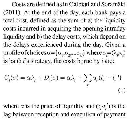r with urgency u. For a given outcome, liquidity costs (first element in Equation 1) depend linearly on liquidity cost α and delay costs (second ele­ment in Equation 1) depend linearly on payment urgency u_r. The dependence of total costs C_i on τ_i and on ‘others’ choices σ_j comes via the delays (t_r-t'), which depend on the τ^,s and λ's of all banks in the system.

Equilibrium

The model has N players, actions λ_i and τ_i for each player and costs (payoffs) determined as described in the above section. We concentrate 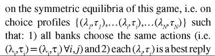to others’ choices. As usual, an ‘equilibrium’ is a strategy profile such that any unilateral deviation is not beneficial to the deviator-even if it would lead to a non-symmetric outcome.

By restricting attention to symmetric equilib­ria, we may miss equilibria where banks adopt different, albeit mutually optimal, choices. Our focus on symmetric equilibria is mainly dictated by simplicity reasons. However, extra-model con­siderations suggest that such asymmetric equilibria (should they exist) would be unlikely to survive in reality. First, if a bank posted less liquidity than others, it might be seen to ‘free-ride’ and could be somehow sanctioned in the long run. Second, in reality banks do not know the choices of their counterparties. What they typically do know is some average indicator of the whole system, and this is what they play against. If Nis large, all banks will face the same ‘average opponent,’ and, being identical, they will all choose the same best reply to that. This confirms that symmetric equilibria are the ones to concentrate on here.

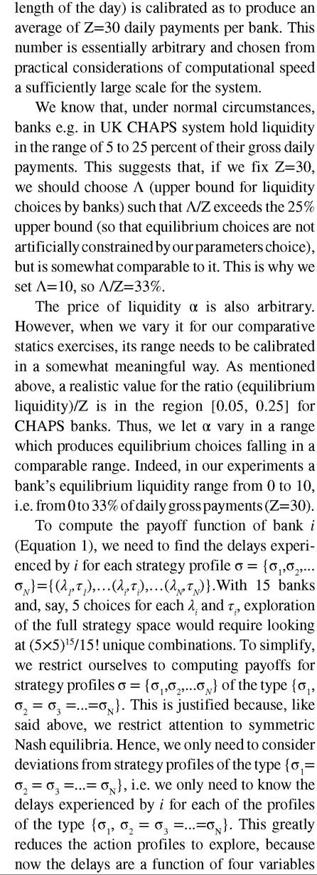
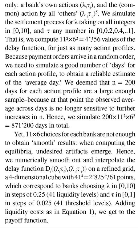
Model Parameters and Payoff Simulations

We use simulations to determine the payoff function. We model a system of 15 banks. The Poisson process for instruction arrival (and thus

RESULTS

We start by analyzing the costs for payment de­lays and then add liquidity costs to arrive at total costs-i.e. the payoff function of the game. Once these are established, we describe the properties of equilibria that arise in a game with such payoffs.

Delay Costs

We start by looking at the delay costs in a plain RTGS system. Figures 1 and 2 show the two com­ponents of delay costs: delays stemming from the RTGS stream, and delays stemming from either delaying payments internally, or delaying them in the LSM stream. The urgency threshold τ is shown

Figure 1. Total delay costs: RTGS with internal queues as a function of threshold. Each chart in the panel represents a given level of liquidity in the system.

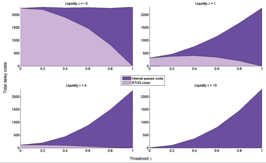
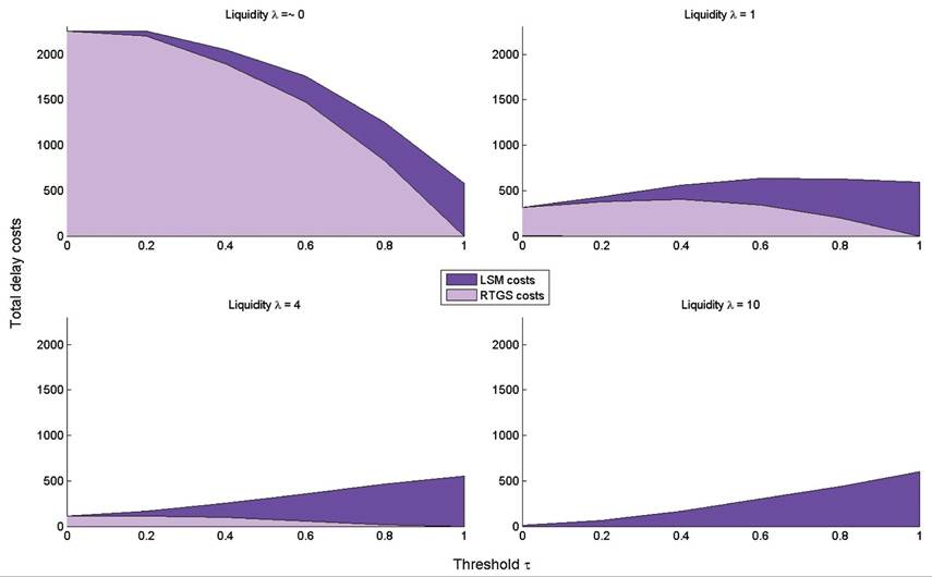
Figure 2. Total delay costs: RTGS with LSM as a function of threshold. Each chart in the panel represents a given level of liquidity in the system.

in each panel on the horizontal axis; the vertical axis shows the delay costs. The four panels are for increasing levels of liquidity chosen by the banks.

When banks have almost no liquidity (Figure 1, top left), no settlement takes place and pay­ments are delayed either in RTGS queue or held internally at the banks. When liquidity is increased (top right), settlement can take place in the RTGS stream. As more payments are held internally (i.e. as the threshold τ grows), the costs stemming from delays in the RTGS stream rise, reason being that the liquidity efficiency of the RTGS system is reduced, so more delays accumulate there. The same of course holds for internal queues’ delays (as more payments are indeed queued internally). From a certain point on though (when τ~0.4), RTSG delays (and the associated costs) start to fall. This is because RTGS payments become so few, that even if they settle rather slowly, their number is limited, so the effect on the product (delays)?(number of delayed payments) actually falls. In the limit, as τ = 1, no payments are sent to the RTGS stream, so no delays accumulate there. With higher level of liquidity, the mechanisms at work are exactly identical, except that RTGS delays are smaller.

A LSM stream can reduce delays substantially. When all payments are settled using the LSM stream (τ = 1), the amount of liquidity λ present in the system is irrelevant (indeed, liquidity is only used in the RTGS stream). In this case, delays are around one fifth of those suffered when the LSM is not available.. By the same token, the delays in the LSM stream are not affected by the amount of liquidity, but only by τ, i.e. by the share of pay­ments submitted to the LSM. So when liquidity is increased, delays in the RTGS stream are reduced, while delays in the LSM stream are unaffected. However, just like the RTGS stream, the LSM stream is more efficient when more payments are submitted to it⁶.

Total Costs

Total costs are obtained by adding liquidity costs to delay costs, as discussed before (Equation 1). In turn, delay costs depend on the liquidity and threshold choices by all banks. Figure 3 refers to a system with an LSM. Taking the point of view of a single bank, it shows how ‘my’ total costs depend on ‘my’ choices, for various ‘others’ choices-which of course may be different from ‘my’ choices.

The pictures in the first row show the impact of ‘my’ choices when ‘others’ liquidity is low. The second row shows the consequences of ‘my’ choices when ‘others’ liquidity is high. Moving left to right along a row, the ‘others’ threshold is increased. These figures show that the depen­dence of ‘my’ payoffs on ‘my’ choices varies dramatically. For example, when others provide little liquidity and route most payments to RTGS (Figure 2, top-left), my total costs are minimized by routing all my payments to RTGS, providing somewhat more liquidity than the others. So, in a sense, I would be forced to give in and provide liquidity, if others do not. On the other hand, if other banks provide large amounts of liquidity and route half of payments to RTGS (bottom-middle), I should provide no liquidity at all (others already do so sufficiently) and I should route most pay­ments to RTGS, according to the well-known ‘free-riding’ strategy.

This shows that the basic structure of a ‘plain’ RTGS liquidity game (whereby there are incen­tives to free-ride, but if others do so, I should accommodate) is preserved in this more complex setting. However, as we will see in what follows, the presence of the LSM softens these incentives, making it possible to achieve better equilibrium outcomes.

The efficiency of each stream (RTGS or LSM) depends on the share of payments routed to it by the ‘others’ (i.e. by their threshold). In addition,

Figure 3. ‘My’ costs for different choices by ‘others’-with LSM

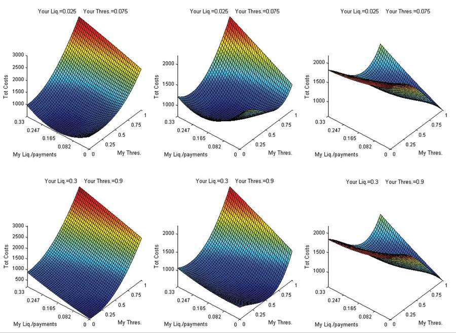
the efficiency RTGS stream also depends on the amount of liquidity committed by ‘others’: the more liquidity ‘others’ post, the more attractive the RTGS becomes, as ‘my’ liquidity and ‘others’ liquidity are complements.

Equilibria

As mentioned earlier, we concentrate on symmet­ric equilibria, i.e. action profiles where all banks make the same choices. To find these, we look for fixed points of the best reply correspondence. That is, for each choice by the ‘others,’ we compute ‘my’ optimal choice of τ and λ, and then look for choices, which are best replies to themselves.

A key parameter in the model is the price of liquidity α in Equation 1. This is arguably the vari­able over which central banks and policy makers have the greatest influence. Thus we look at how the equilibrium varies when the price of liquidity α changes. An accurate calibration of the model is beyond the scope of this chapter. Thus, we let the parameter α vary in a range wide enough for the equilibria to span the whole strategy space­keeping the price of delays fixed.

RTGS with Withholding Payments

Figure 4 shows equilibria and the planner’s choices for different prices of liquidity. Equilibrium choices are represented by dots, while the planner’s choices are represented by stars. The background gradient shows system-wide costs, which are, by definition, lowest at the planner’s choice.

Figure 4. Equilibria and planner’s choices without LSM. Each chart refers to a given price of liquidity (lowest price on top-left; highest price on bottom-right).

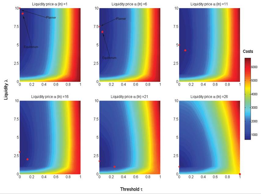
The planner's choice of τ is dichotomous. Either all payments are sent to RTGS, or they are all internally queued until the end of the day. Equilibrium choices are less stark, and banks typically use both queues and RTGS. When the (relative) price of liquidity rises, banks post less liquidity and resort to delaying payments inter­nally. Importantly, the equilibrium is inefficient: a cost-minimizing planner would provide more liquidity to the system and would never delay payments internally. Equilibrium costs are always more than 15% higher than the social optimum, reaching multiples thereof at high liquidity prices. Only when the price of liquidity is extremely high, the equilibrium coincide with the planner's optimal choice, both being {λ=0, τ=1}.

The reason for this inefficiency is explained by two externalities. On the one hand, there is a positive externality in liquidity provision: in­coming payments to a bank can be recycled for making other payments, so liquidity is in a sense a common good, as in Angelini (1998). As a result, equilibrium liquidity provision (λ) falls short of the social optimum. On the other hand, internal queues generate a negative externality: banks have an incentive to delay less urgent payments, and use liquidity for more urgent ones. However, by doing so, they slow down the beneficial liquidity recycling in RTGS, which in turn affects other banks. Hence, banks queue more than they should from a social perspective-i.e. τ exceeds the level that would be chosen by the planner.

RTGS with LSM

As with internal delays of payments, the routing of payments to a LSM allows banks to reserve liquidity for urgent payments in RTGS. However, while internal queues merely postpone settle­ment until the end of the day, the LSM allows for settlement as soon as offsetting cycles are found, without making use of liquidity. Thus from the outset, the LSM offers a more efficient way of queuing payments.

However, increased efficiency of the second stream induces banks to use it more intensely. In addition, an increase in τ causes a reduction in RTGS volumes, which in turn causes this stream to lose in efficiency. Hence, there is a trade-off between the efficiency levels of the two streams. When ‘played with' by individual banks, these effects may produce unexpected outcomes, as we show next.

Figure 5 shows that, when liquidity costs change, the equilibria change essentially as in the RTGS with internal queues model. In particular, as the price of liquidity (α) rises, liquidity provision (λ) decreases and usage of the LSM (τ) increases. Compared to the social optimum, liquidity provi­sion is too low and payments are delayed too much. For very high prices of liquidity, both banks and the planner rely exclusively on the LSM. Only then is the equilibrium efficient. The planner never uses both streams at the same time-as was already discussed.

Figure 5. Equilibria and planner’s choices for a system with LSM. Each chart refers to a given liquidity price α (lowest α on top-left; highest α on bottom-right).

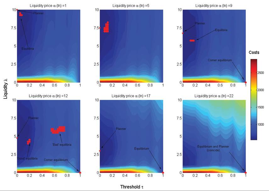
The main novelty with an LSM compared to internal queues is that, for an intermediate range of liquidity costs, multiple equilibria emerge (shown in the picture as separate clusters of ε-equilibria⁷). In a typical case, there are up to three equilibrium types:

1. A corner equilibrium λ=0, τ=1 (all payments via LSM);

2. Equilibria with moderate use of both liquidity and LSM (‘good equilibria’).

3. Equilibria with high usage of both liquidity and LSM (‘bad equilibria’).

Equilibria under (a) are socially optimal (i.e. coincide with the planner’s choice) only in the extreme circumstances of very high liquidity costs. However, they are typically better than the equilibria under (c). These latter are called ‘bad’ as they feature the highest costs among all equilibria. Equilibria under (b) are typically those with lowest costs, so we call them ‘good.’

Although ‘bad,’ the equilibria under (c) are interesting for their paradoxical features: high liquidity usage (λ) and high reliance on the LSM (τ). Their existence is probably explained as fol­lows. LSM features economies of scale, so its high usage may be self-sustaining. However, as mentioned at the start of this section, over-use of the LSM is detrimental to the RTGS stream, which may in turn require inefficiently high amounts of liquidity.

CONCLUSION

We presented in this chapter a model of two styl­ized payment systems. In both of them, banks can queue non-urgent payments to reserve liquidity for urgent ones. In the first system, queued pay­ments are held internally by the banks and are submitted for settlement at the end of the day. In the second system, queued payments are routed to an LSM and are settled throughout the day by an offsetting algorithm.

As expected, the LSM is more efficient than decentralized queuing: it pools otherwise seg­regated queues, allowing continuous settlement throughout the day (Figure 1 and Figure 3). However, more importantly, an LSM changes the strategic interaction between banks, modifying their incentives.

To assess the effects of an LSM from a welfare point of view, we first look at the choices of a social planner, whose objective is to minimizing total costs for the system. When only internal queues are available, the planner willingly delays payments (sets τ < 0) only when liquidity is very expensive (Figure 5). In all other circumstances, the planner submits all payments to the RTGS stream. The planner makes a similar dichotomous choice if it can use an LSM: its sends payments in the LSM only if liquidity exceeds a certain level; otherwise, is settles all payments via the RTGS stream. Thus, from the planner’s perspective, a LSM is only valuable in extreme circumstances.

When looking at banks acting strategically, more complex behavior emerges in equilibrium: for a range of liquidity prices, banks use both direct RTGS settlement and queues (be these internal queues or the LSM). As to be expected, they also queue more at higher liquidity costs. In equilibrium, banks under-provide liquidity and suffer both higher delays and overall costs than socially optimal: the ‘central planner’ would only use the RTGS stream and provide it with more liquidity than the banks do. This inefficiency is due to the fact that banks tend to free-ride on each others’ liquidity.

However, a system with an LSM is capable of delivering better outcomes than those resulting in the absence of a LSM. Indeed, for a range of liquidity prices, we find ‘good’ LSM equilibria, which feature lower total costs than their non- LSM counterparts. Cost savings here derive from faster settlement and often, although not always, to lower liquidity usage.

Our results point out a caveat, though: for a range of liquidity prices, a system with a LSM may also generate ‘bad’ equilibria with 1) high liquidity usage, 2) intense use of the LSM, and 3) high costs, exceeding those obtained without LSM. The exis­tence of these (somewhat paradoxical) equilibria is explained as follows. The LSM stream features economies of scale: the more payments are sent in it, the more efficient the stream becomes. Hence, its high usage may be self-sustaining. However, the RTGS stream also features economies of scale, which is to say: if many payments are sent to the LSM stream, the RTGS stream may become less efficient. Because of this, it may require high amounts of liquidity, which lead to an overall cost­inefficiency. This suggests that liquidity saving mechanisms can be useful, but they may need some coordination device, to ensure that banks arrive at a ‘good’ equilibrium.

ACKNOWLEDGMENT

The views expressed in this chapter are those of the authors, and not necessarily those of the Bank of England. The authors thank participants in: the 6th Bank of Finland Simulator Seminar (Helsinki, 25-27 August 2008); the 1st ABM-BaF confer­ence (Torino, 9-11 February 2009); and the 35th Annual EEA Conference (New York, 27 Febru­ary-1 March 2009). The authors are also indebted to Marius Jurgilas, Ben Norman, Tomohiro Ota, and other colleagues at the Bank of England for useful comments and encouragement. Kimmo Soramaki gratefully acknowledges the support of OP-Pohjola-Ryhman tutkimussaatio.

REFERENCES

Angelini, P. (1998). An analysis of competitive externalities in gross settlement systems. Journal of Banking & Finance, 22, 1-18. doi:10.1016/ S0378-4266(97)00043-5

Bech, M., Preisig, C., & Soramaki, K. (2008). Global trends in large value payment systems. Federal Reserve Bank of New York Economic Policy Review, 14(2), 59-81.

Bech, M., & Soramaki, K. (2002). Liquidity, gridlocks and bank failures in large value payment systems. In E-Money and Payment Systems Re­view. London, UK: Central Banking Publications. Beyeler, W., Bech, M., Glass, R., & Soramaki, K. (2007). Congestion and cascades in payment sys­tems. Physica A, 384(2), 693-718. doi:10.1016/j. physa.2007.05.061

Buckle, S., & Campbell, E. (2003). Settlement bank behavior and throughput rules in an RTGS payment system with collateralised intraday credit. Bank of England Working Paper no. 209. London, UK: Bank of England.

Galbiati, M., & Soramaki, K. (2011). An agent­based model of payment systems. Journal of Economic Dynamics & Control, 35(6), 859-875. doi:10.1016/j.jedc.2010.11.001

Guntzer, M. M., Jungnickel, D., & Leclerc, M. (1998). Efficient algorithms for the clearing of interbank payments. European Journal of Op­erational Research, 106, 212-219. doi:10.1016/ S0377-2217(97)00265-8

Johnson, K., McAndrews, J. J., & Soramaki, K. (2004). Economizing on liquidity with deferred settlement mechanisms. Federal Reserve Bank of New York Economic Policy Review, 10(3), 51-72.

Leinonen, H. (Ed.). (2005). Liquidity, risks and speed in payment and settlement systems - A simulation approach. Bank of Finland Studies. Helsinki, Finland: Bank of Finland.

Leinonen, H. (Ed.). (2007). Simulation studies of liquidity needs, risks and efficiency in payment networks. Bank of Finland Studies. Helsinki, Finland: Bank of Finland.

Leinonen, H. (2009). (Ed.). Simulation analyses and stress testing of payment networks. Bank of Finland Studies. Helsinki, Finland: Bank of Finland.

Martin, A., & McAndrews, J. J. (2008). Liquid­ity-saving mechanisms. Journal of Monetary Economics, 55(3), 554-567. doi:10.1016/j. jmoneco.2007.12.011

Shafransky, Y. M., & Doudkin, A. A. (2006). An optimization algorithm for the clearing of interbank payments. European Journal of Opera­tional Research, 171(3), 743-749. doi:10.1016/j. ejor.2004.09.003

Willison, M. (2005). Real-time gross settlement and hybrid payments systems: A comparison. B ank of England Working Paper no. 252. London, UK: Bank of England.

ADDITIONAL READING

Adams, M., Galbiati, M., & Giansante, S. (2010). Liquidity costs and tiering in large-value payment systems. Bank of England Working Paper 399. London, UK: Bank of England.

Angelini, P., Maresca, G., & Russo, D. (1996). Sys­temic risk in the netting system. Journal of Bank­ing & Finance, 20, 853-868. doi:10.1016/0378- 4266(95)00029-1

Bech, M. L., & Garratt, R. (2003). The intraday liquidity management game. Journal ofEconomic Theory, 109(2), 198-219. doi:10.1016/S0022- 0531(03)00016-4

Bech, M. L., & Soramaki, K. (2005). Systemic risk in a netting system revisited. In H. Leinonen (Ed.), Liquidity, Risks and Speed in Payment and Settlement Systems - A Simulation Approach (pp. 275-296). Helsinki, Finland: Bank of Finland. Becher, C., Millard, S., & Soramaki, K. (2008). The network topology of CHAPS sterling. Bank of England Working Paper 355. London, UK: Bank of England.

Boss, M., Krenn, G., Metz, V., Puhr, C., & Schmitz,

S. W. (2008). Systemically important accounts, network topology and contagion in ARTIS. OeNB Financial Stability Report 15. OeNB.

Fudenberg, D., & Levine, D. K. (1998). The theory of learning in games. Cambridge, MA: MIT Press.

Galbiati, M., & Giansante, S. (2010). Emergence of networks in large value payment systems. DEPFID Working Paper 1/2010. DEPFID.

Galos, P., & Soramaki, K. (2005). Systemic risk in alternative payment system designs. European Central Bank Working Paper 508. Hesse, Ger­many: European Central Bank.

Haldane, A. (2009). Rethinking the financial network. Paper presented at the Financial Student Association. Amsterdam, The Netherlands.

Humphrey, D. (1986). Payments finality and risk of settlement failure. In A. Saunders, & L. J. White (Eds.), Technology and the Regulation of Financial Markets: Securities, Futures, and Banking (pp. 97-120). Lexington, MA: Heath.

Kokkola, T. (Ed.). (2010). The payment system. Frankfurt, Germany: European Central Bank.

Koponen, R., & Soramaki, K. (1998). Intraday liquidity needs in a modern interbank payment system - A simulation approach. Bank of Finland Studies in Economics and Finance 14. Helsinki, Finland: Bank of Finland.

Leinonen, H., & Soramaki, K. (1999). Optimizing liquidity and settlement speed in payment systems. Bank of Finland Discussion Paper 16. Helsinki, Finland: Bank of Finland.

Manning, M., Nier, E., & Schanz, J. (Eds.). (2009). The economics of large-value payments and settle­ment: Theory and policy issues for central banks. Oxford, UK: Oxford University Press.

Martinez-Jaramillo, S. (2007). Artificialfinancial markets: an agent based approach to reproduce stylized facts and to study the red queen effect. Essex, UK: University of Essex.

Martinez-Jaramillo, S., & Tsang, E. P. K. (2009). An heterogeneous, endogenous and co-evolution- ary GP-based financial market. IEEE Transactions on Evolutionary Computation, 13(1), 33-55. doi:10.1109/TEVC.2008.2011401

Renault, F., Beyeler, W. E., Glass, R. J., Soramaki,

K., & Bech, M. L. (2009). Congestion and cas­cades in interdependent payment systems. Sandia National Laboratories Working Paper 2009-2175. Albuquerque, NM: Sandia National Laboratories.

Soramaki, K., Bech, M., Arnold, J., Glass, R. J., & Beyeler, W. E. (2007). The topology of interbank payment flows. Physica A: Statistical Mechanics and its Applications, 379(1), 317-333.

Intraday Liquidity: Funds available for set­tling payments. These consist normally of reserve balances and intraday credit extended from the central bank.

Liquidity Risk in Payment Systems: The risk that lack of funds prevents the settlement of payments longer than preferred by the bank.

Liquidity Saving Mechanisms (LSM): Al­low payment settlement with less liquidity by enhancing participating bank’s coordination on the timing of payment submission or by synchro­nizing timing of settlement so that payments can offset each other.

Real Time Gross Settlement (RTGS) Sys­tems: Are funds transfer systems where the transfer of funds takes place from one bank to another on continuous (real time) basis and where each payment is processed individually (gross) only if sufficient cover is available on the sending bank’s account.

Settlement Risk in Payment Systems: The risk that arises when a payment has been credited to the account of the recipient before full cover has been transferred by sending bank. RTGS settlement eliminates settlement risk.

KEY TERMS AND DEFINITIONS

Circles Processing: An algorithm that searches for subsets of payments that could be settled simultaneously with the funds available to each bank which consist of external liquidity and funds received from payments in the algorithm’s solution.

Gridlock: A situation where several payments await the settlement of each other but none can be settled with existing allocation of funds among the sending banks. See circles processing.

Interbank Payment System: A system op­erated by the central bank that allows financial institutions to transfer claims on central bank money, or ancillary systems that settle in central bank operated payment systems.

ENDNOTES

e.g. ‘The European Interbank Guidelines on Liquidity Management’ by the European Banking Federation (EBF) or ‘Throughput Guidelines’ in the CHAPS system rules. A problem in combinatorial optimization, which derives its name from the problem faced when packing a rucksack of limited size with valuable obj ects-so as to maximize the total value of objects fitting in it.

RRGS bases the settlement of queued pay­ments on the value of incoming payments rather than on a participant’s account bal­ance-providing enhanced incentives to submit payments for settlement earlier.

Larger banks usually employ software algorithms to release payments based on estimates on the bank’s liquidity position on the given day and on future days. The schedulers may contain limits for bilateral positions, buffers for unexpected events, and are tied with the bank’s end of day liquidity management in the interbank lending market. Smaller banks release payments individually and manually.

Galbiati and Soramaki (2011) show that, in a simpler game where banks choose only the amount of liquidity to settle payments, all that matters for a bank are its own liquidity and the average (sum) of others’ liquidity (in technical terms, they show that the liquidity game is a potential game). This suggests that concentrating on strategy profiles of the kind {σ₁, σ₂ = σ₃ =...=∏_n} may be not so restrictive as it could seem at first.

Total delays can be calculated as x∙(τ∕2)∙τ, where x is the average time delayed, (τ∕2) the average urgency and τ the volume routed to RTGS. Simulations show that total delays scale as α∙τ, so one deduces that x~α∙1∕τ. In a sense, LSM displays increasing returns to scale with respect to processed volumes. The larger the pool of payments on which an LSM searches for cycles, the more likely (and longer) will be the cycles themselves. An ε-equilibrium is a strategy profile from which deviation yields at most a small (ε) gain to the deviator. Here it is simpler to compute and visualize ε-equilibria (instead of plain equilibria) because our numerical results are obtained on finite ‘grids’ in the (λ, τ)² space.

This work was previously published in Simulation in Computational Finance and Economics, edited by Biliana Alexandrova- Kabadjova, Serafin Martinez-Jaramillo, Alma Lilia Garcia-Almanza, and Edward Tsang, pages 103-119, copyright 2013 by Business Science Reference (an imprint of IGI Global).