Chapter 77 The Use of Soft Computing for Optimization in Business, Economics, and Finance
Petr Dostal
Brno University of Technology, Institute of Informatics, Czech Republic
ABSTRACT
Optimization methods have had successful applications in business, economics, and finance.
Nowadays the new theories of soft computing are used for these purposes. The applications in business, economics, and finance have specific features in comparison with others. The processes are focused on private corporate attempts at money making or decreasing expenses; therefore the details of applications, successful or not, are not published very often. The optimization methods help in decentralization of decision-making processes to be standardized, reproduced, and documented. The optimization plays very important roles especially in business because it helps to reduce costs that can lead to higher profits and to success in the competitive fight.1. INTRODUCTION
There are various optimization methods appropriate to use in business and economics: classical ones and methods using soft computing such as fuzzy logic, neural networks, genetic algorithms, and the theory of chaos.
Soft computing differs from conventional (hard) computing in that, unlike hard computing, it is tolerant of imprecision, uncertainty, partial truth, and approximation. In effect, the role model for soft computing is the human mind. The guiding principle of soft computing is: Exploit the tolerance for imprecision, uncertainty, partial truth, and
DOI: 10.4018∕978-1-4666-6268-1.ch077 approximation to achieve tractability, robustness and low solution cost. The basic ideas underlying soft computing in its current incarnation have links to many earlier influences, among them Zadeh’s 1965 paper on fuzzy sets. The inclusion of neural computing and genetic computing in soft computing came at a later point.
At this juncture, the principal constituents of Soft Computing (SC) are Fuzzy Logic (FL), Neural Computing (NC), Evolutionary Computation (EC) Machine Learning (ML) and Probabilistic Reasoning (PR), with the latter subsuming belief networks, chaos theory and parts of learning theory.
What is important to note is that soft com-.
puting is not a melange. Rather, it is a partnership in which each of the partners contributes a distinct methodology for addressing problems in its domain. In this perspective, the principal constituent methodologies in SC are complementary rather than competitive. Furthermore, soft computing may be viewed as a foundation component for the emerging field of conceptual intelligence.
The mentioned applications in this chapter are as follows:
• Risk investment
• Risk management (loans, mortgages, direct mailing)
• Optimization of number of objects (devices, stock)
• Prediction of time series
• Journey optimization
• Description of economic phenomena
(stock market).
The program MATLAB® with Fuzzy Logic, Neural Network, and Global Optimization Toolbox is used. The fields of applications of optimization methods in business, economics, and finance cover a wide area of applications.
2. FUZZY LOGIC
2.1 Fundamentals of Fuzzy Logic
In classical logic, a theory defines a set as a collection having certain definite properties. Any element belongs to the set or not according to clear-cut rules; membership in the set has only the two values 0 or 1. Later, the theory of fuzzy logic was created by Zadeh in 1965. Fuzzy logic defines a variable degree to which an element x belongs to the set. The degree of membership in the set is denoted μ(x); it can take on any value in the range from 1 to 0, where 0 means absolute non-membership and 1 full membership. The use of degrees of membership corresponds better to what happens in the world of our experience. Fuzzy logic measures the certainty or uncertainty of how much the element belongs to the set. People make analogous decisions in the fields of mental and physical behaviour. By means of fuzzy logic, it is possible to find the solution of a given task better than by classical methods.
The fuzzy logic system consists of three fundamental steps: fuzzification, fuzzy inference, and defuzzification (see Figure 1).
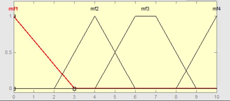
The first step (fuzzification) means the transformation of ordinary language into numerical values. For variable risk, for example, the linguistic values can be no, very low, low, medium, high, and very high risk. The variable usually has from three to seven attributes (terms). The degree of membership of attributes is expressed by mathematical functions. There are many shapes of membership functions. For example, for mf1, P = [0 0 3]; mf2, P = [2 4 6]; mf3, P = [4 6 7 9]; mf4, P = [8 10 10]; and so forth (see Figure 2).
The types of membership functions that are used in practice are for example Λ and Π. There are many other types of standard membership functions on the list including spline ones. The attribute and membership functions concern input and output variables.
The second step (fuzzy inference) defines the system behaviour by means of the rules such as,,. The conditional
Figure 1 Decision making solved by means of fuzzy logic

Figure 2. The types of membership functions Λ and Π
clauses create this rule, which evaluates the input variables. These conditional clauses have the form
I1 is mf I2 is mfb... In 1 is mf In is mf O1 is mfO1 s".
The written conditional clause could be described by words: If the input I1 is mfa or I2 is mfb or... or IN_ 1 is mf or In is mf then O1 is mfO1 with the weight s, where the value s is in the range. These rules must be set up and then they may be used for further processing.
The fuzzy rules represent the expert systems. Each combination of attribute values that inputs into the system and occurs in the condition,, represents one rule.
Next it is necessary to determine the degree of supports for each rule; it is the weight of the rule in the system. It is possible to change the weight rules during the process of optimization of the system. For the part of rules behind, it is necessary to find the corresponding attribute behind the part. These rules are created by experts. The could be instead.The third step (defuzzification) means the transformation of numerical values to linguistic ones. The linguistic values can be, for example, for variable Risk very low, low, medium, high, and very high. The purpose of defuzzification is the transformation of fuzzy values of an output variable so as to present verbally the results of a fuzzy calculation. During the consecutive entry of data the model with fuzzy logic works as an automat. There can be a lot of variables on the input.
The chapter is focused on applications. The fuzzy theory is described in books such as (Altroc 1996), (Dostal 2011), (Chen et al. 2004), (Chen et al. 2007), (Kazabov and Kozma 1998), (Klir and Yuan 1995), (Li et al. 2006), (The MathWorks 2010b).
2.2 Applications of Fuzzy Logic
Example 2.1: The Fuzzy Logic Toolbox enables setting up rules by means of neural networks using the command Anfis. The setup of fuzzy rules in the program environment MATLAB with the help of neural networks is presented for a case study, where the program creates the fuzzy rules by means of neural networks. The inputs and outputs are defined by Table 1, presenting the logical operation. We demonstrate four states. The first state represent the fact that the political risk is high (0) and economic risk is high (0) and it leads to state of output of no investment (0). The second state represent the fact that the political
risk is high (0) and economic risk is low (1) and it leads to state of output of no investment (0). The third state represent the fact that the political risk is low (1) and economic risk is high (0) and it leads to state of output of no investment (0).
The fourth state represent the fact that the political risk is low (1) and economic risk is low (1) and it leads to state of investment (1).The text file Risk.dat is created with the mentioned data at first (Table 2).
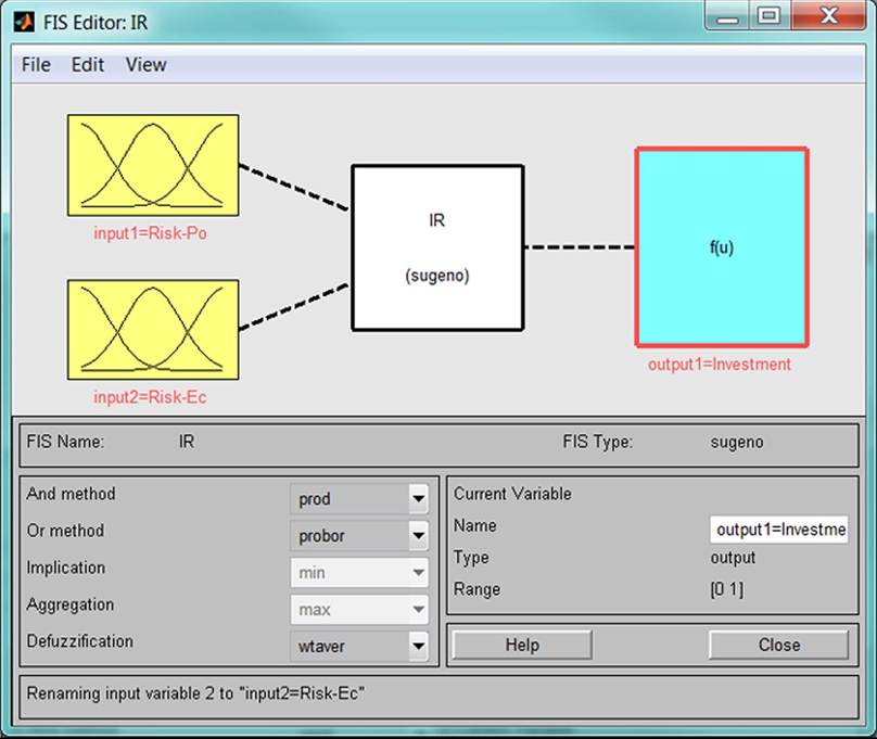
The commands//./-~v and File-New FlS-Sugeno create a fuzzy model in the MATLAB environment, then there follow commands Edit-Add Variable-Input that add the second input. The fuzzy model is saved in lR.fis file (see Figure 3).
Table 1. The input and output values
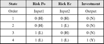
Table 2. Input and output values
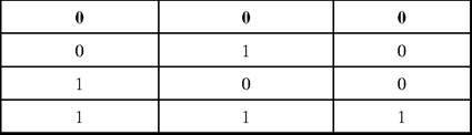
Figure 3. Fuzzy model
The command Edit-Anfis opens the editor. The choice of menu Type-Training and From-file and command Load-Data read the file Risk.dat (see Figure 4).
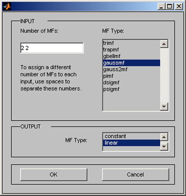
The Fuzzy Interface System is generated from the command FIS with the option Grid partition. It is set up with the numbers of two membership functions for both inputs Number of MF’s [2 2], then the Gaussian membership function is set up from the commands MF Type gaussmf and linear type MF Type - linear. The return is done by the OK menu (see Figure 5).
The values for training of neural networks create the rules chosen by options Optim. MethodHybrid, Error Tolerance 0, and the number of Epochs 20. The process of training starts with the command Train Now. It is desirable to watch the error training (see Figure 6).
The command Structure shows the created neural network used for generation of rules (see Figure 7).
The command TestFIS - Training data enables comparing trained data with the real ones, possibly with testing and checking data (see Figure 8).
The dependence of outputs on input can be displayed by standard commands (see Figure 9). The surface reflects the proper generation of rules.
It is possible to display the generated rules (see Figure 10).
The command Rules enables the verification of created rules (see Figure 11).
The presented case study describes the methodology of creation of rules by means of neural networks using the data from databases. The problem could involve complicated tasks, where a large number of rules are created. If the rules
Figure 4. Reading of data and their display
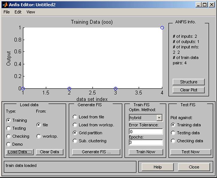
Figure 5. The setup of membership functions
could not describe the solved problem successfully, the displayed surface shows “disturbances.” In the case of wrong generalization, the trained model does not correspond with new data.
The advantage of the use of fuzzy logic in comparison with classical methods is in the fact that vague terms could be processed by fuzzy decision making model. This example presents risk of investment. More inputs are generally used.
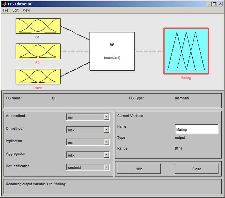
Example 2.2: There are situations when more rule boxes are necessary for using the decisionmaking process and for their connection. The connection can be done by creation of an M-file that enables reading the input data, but also the transfer of results to other blocks. The case presents the use of fuzzy logic at direct mailing, whether the client visit personally, sent him a letter or not to speak to him (see Figure 12).
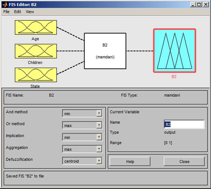
The input variables in block B1 (Figure 13) and their attributes are Loan I1a (none, small, medium, high) and Salary I (low, medium, high). The input variables in block B2 (Figure 14) and their attributes are Age Ib (young, medium, old, very old), Children Ib (no, a few, many) and State Ib (single, married, divorced). The input variables in block Bf (Figure 15) and their attributes are Place I3 (big city, city, village). The rule blocks with attributes are Finance (excellent, good, bad),
Figure 6. Anfis editor-error training
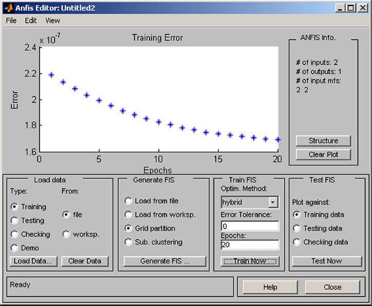
Figure 7. Created neural network
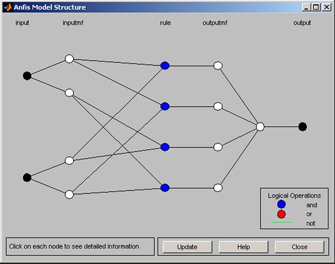
Figure 8. Evaluation of training
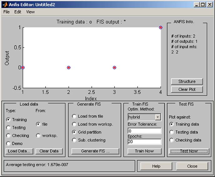
Figure 9. Dependence of output on inputs
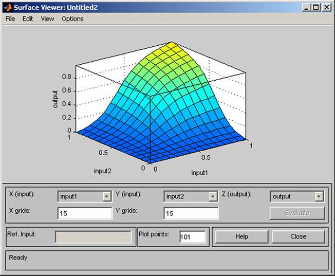
Figure 10. Generated rules
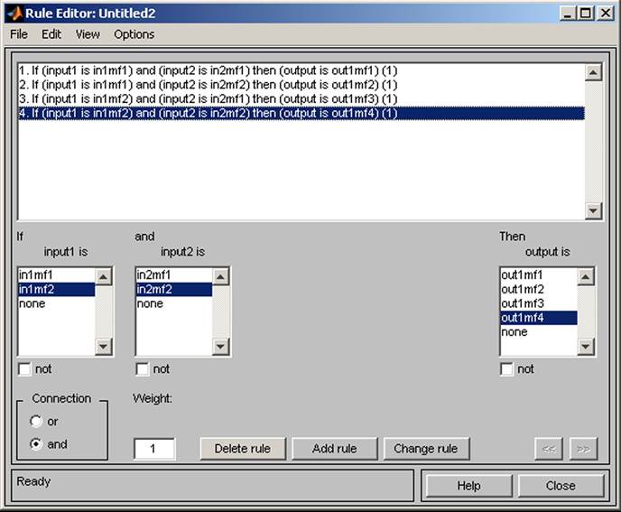
Figure 11. Verification of rules
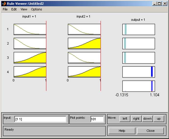
Figure 12. Connection of rule blocks
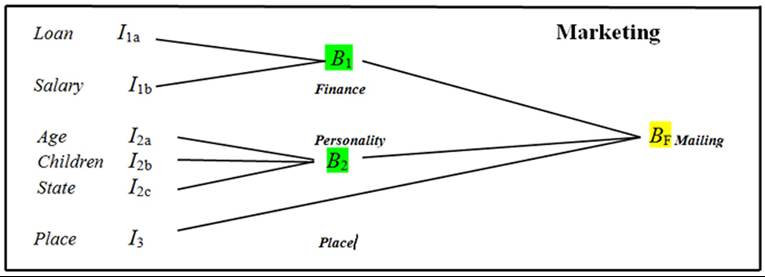
Personality (unsuitable, suitable, good, excellent); and output Mailing (inactivity, mail, personally).
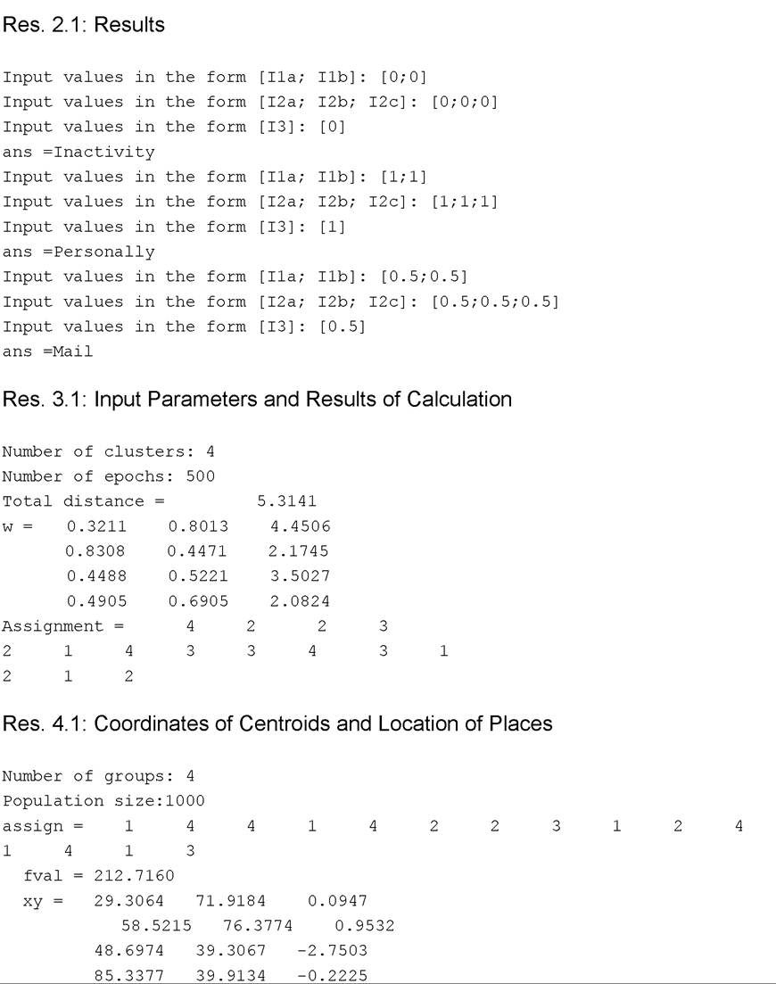
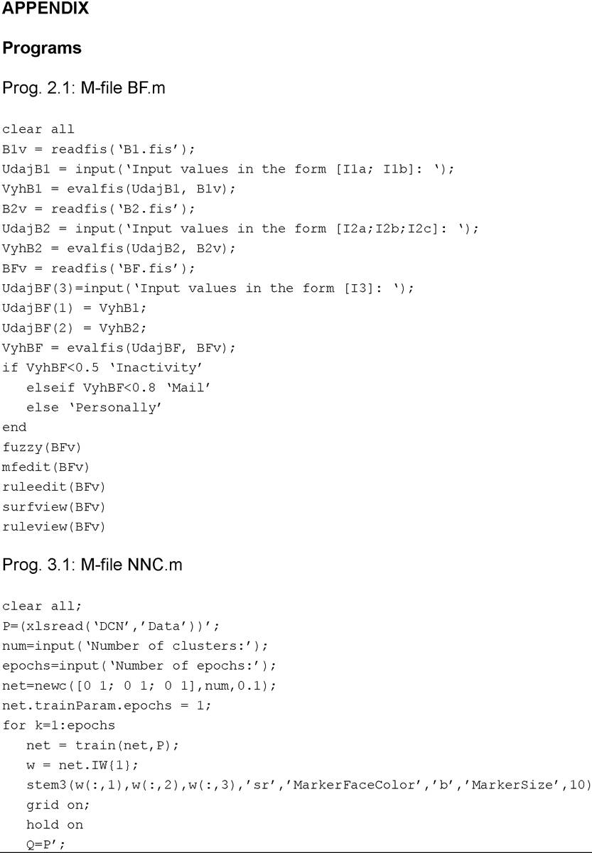
The M-file BF.m (Prog. 2.1 in the Appendix) provides the calculation. The results of the calculation (Results 2.1 in the Appendix) are presented by inputs I1λ, I1b, I2a, I2b, I2c, I3 with values 0, 1, and 0.5. The results are the attributes Inactivity (client will not be spoken), or Personally (client will be visited), or Mail (a letter will be sent to him).
The advantage of fuzzy logic is in the use when values can be described only by vague terms in comparison with classical methods. The vague
Figure 13. Box B1

Figure 14. Box B2
terms could be processed by fuzzy decision making model. The example presents the decision making in direct marketing.
3. NEURAL NETWORKS
3.1 Principles of Neural Networks
The history of the development of neural networks started in the first half of the twentieth century. The first publications were by McCulloch. Later Pitts worked on the simplest model of a neuron, and after that Rosenblatt created a functional perception that solves only problems involving areas that are linearly separable. When the multilayer network was discovered by Rumelhart, then Hinton and Williams created back-propagation methods for multi-layer networks. A great boom of neural network applications has been ongoing since the mid-1970s.
The neural network model represents the thinking of the human brains. The model is described as a “black box.” It is not possible to know the inside structure of the system in detail. We make only a few suppositions about the inner structure of the system. It is simulated by a “black box” that enables us to describe the behaviour of the system by the function that performs transformation of input and output. It is suitable to use neural networks in cases where the influences on searched phenomena are random and deterministic relations are very complicated. In these cases we are not able to separate and analytically identify them.
Figure 15. Box Bp
They are suitable for simulation of complicated and often irreversible strategic decision making. The biological neuron can be presented in a simple way that consists of many inputs (dendrites), body (soma), and one output (axon) as shown in Figure 16. The inputs are processed by neurons. The output information is spread by the axon to terminals that are called “synapses.” The synapsis communicates with the dendrites of other neurons.
The history of the development of neural networks started in the first half of the twentieth century. The first publications were by McCulloch. Later Pitts worked on the simplest model of a neuron, and after that Rosenblatt created a functional perception that solves only problems involving areas that are linearly separable. When the multilayer network was discovered by Rumelhart, then Hinton and Williams created back-propagation methods for multi-layer networks. A great boom of neural network applications has been ongoing since the mid-1970s.
The neural network works in two phases. In the first phase the network presents a model of a complicated system as a “curious pupil”; it tries to set up parameters so as to best correspond to the topology of neural networks. In the second phase, the neural network becomes an “expert” to produce the outputs based on the knowledge obtained in the first phase. During the building up of a neural network, the layers of the network must be defined (input, hidden, output); single input and output neurons specified, and the method
Figure 16. The biological neuron
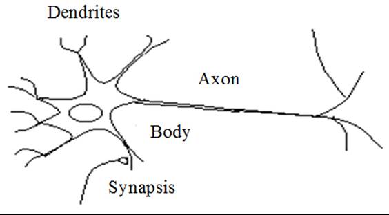
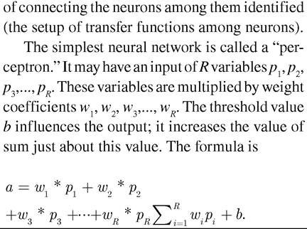
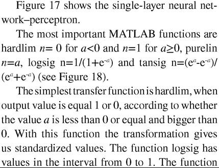
Figure 17. Perceptron
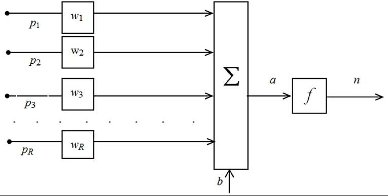
Figure 18. Transfer functions hardlim, purelin, logsig, and tansig
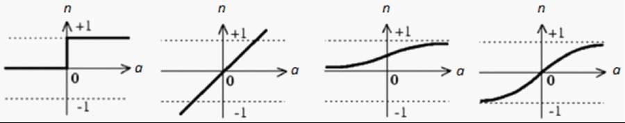
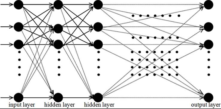
Figure 19. The diagram of multi-layer network
3.1 Applications of Neural Networks
Example 3.1: There are many tasks from business, economics, and finance where clustering helps to make correct decision making. The Kohonen neural network can be used for these purposes. This example describes the method of calculation, how the program is created, and how the case study is applied. The algorithm is as follows: 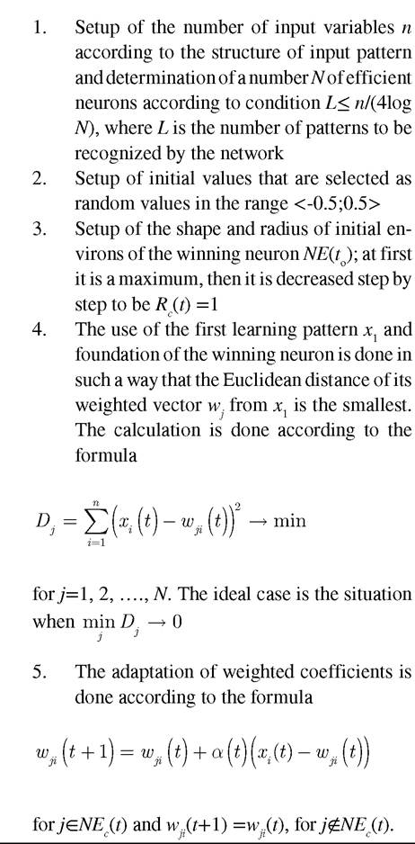
The teaching is continued until the weighted coefficients do not change if a random pattern from the collection of learning patterns is used.
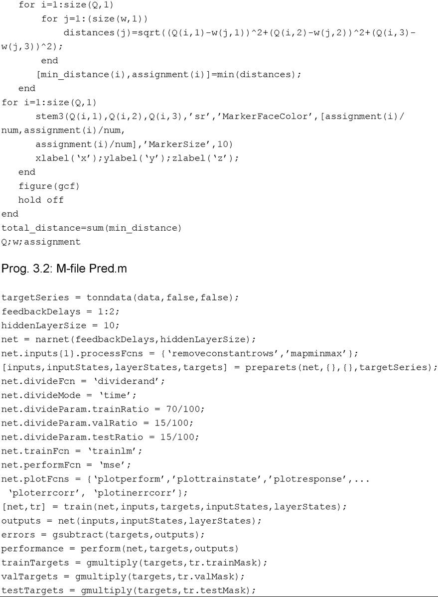
The example presents the objects recorded in MS Excel format in DC.xls file (Table 3). This task is solved by the program NNC.m (Prog. 3.1 in the Appendix).
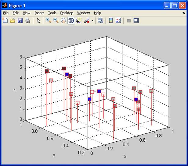
The program is started using the command NNC in the MATLAB program environment. It is necessary to set up the number of clusters, in our example 4 and number epochs 1000. During the process of calculation the data are dynamically displayed in a three-dimensional graph. When the calculation is finished the input parameters and the results of the calculation are presented in the Appendix (Results 3.1).
The results are presented by coordinates of clusters and assignment of objects to the clusters. The two and three-dimensional stem graph is drawn (Figure 20 and Figure 21). The task solves the problem of minimizing the costs of constructions of transmitters of mobile network.
Table 3. Coordinates of objects
| Coordinates of Objects | ||||
| Number | Object | xι | X2 | x3 |
| 1 | Praha | 37 | 72 | 191 |
| 2 | Brno | 72 | 30 | 194 |
| 3 | Ostrava | 100 | 57 | 215 |
| 4 | Plzen | 18 | 60 | 354 |
| 5 | Olomouc | 83 | 42 | 209 |
| 6 | Liberec | 47 | 100 | 402 |
| 7 | Hradec Kralove | 59 | 76 | 231 |
| 8 | Ceske Budejovice | 36 | 24 | 391 |
| 9 | Usti nad Labem | 30 | 99 | 326 |
| 10 | Pardubice | 64 | 67 | 229 |
| 11 | Zlin | 89 | 32 | 330 |
| 12 | Kladno | 30 | 74 | 451 |
| 13 | Opava | 94 | 59 | 255 |
| 14 | Jihlava | 8 | 81 | 525 |
Figure 20. Two-dimensional graph: 4 clusters
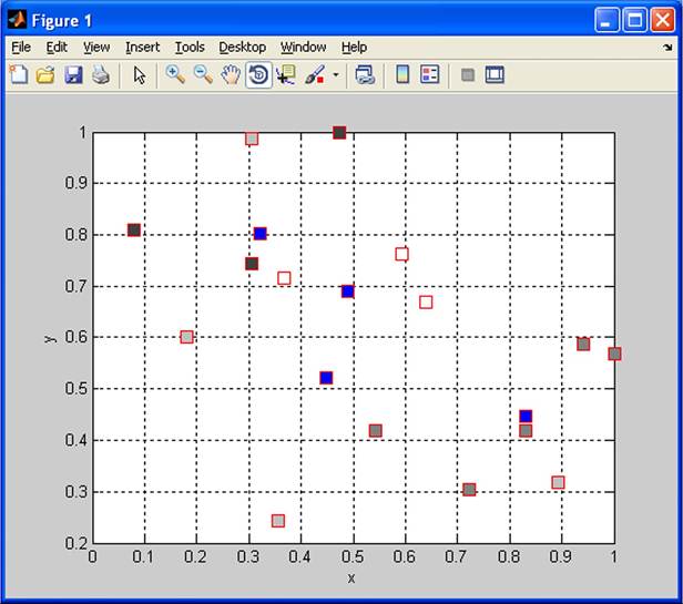
Figure 21. Three-dimensional graph: 4 clusters
The advantage of neural network theory is in successful use of clustering problems that are used quite often in economy and finance.
Example 3.2: The Neural Network Toolbox of MATLAB contains a special toolbox for prediction of time series, which is quite often used in the business and economics. This example presents the prediction of time series from history created by the number of sold products recorded in D.xls file. The menu is called from workspace using the command ntstool. At first, it is necessary to setup the type of neural network. The Nonlinear Autoregressive Model (NAR) was chosen (see Figure 22).
Then it is necessary to click on button Next and download the data from the D.xls file. When the data are downloaded, the window is closed using the command Finish (see Figure 23).
After the data have been selected, as in Figure 24, the command Next opens a window for the setup of Training, Validation, and Testing. The default value can be used or it could be changed (see Figure 25).
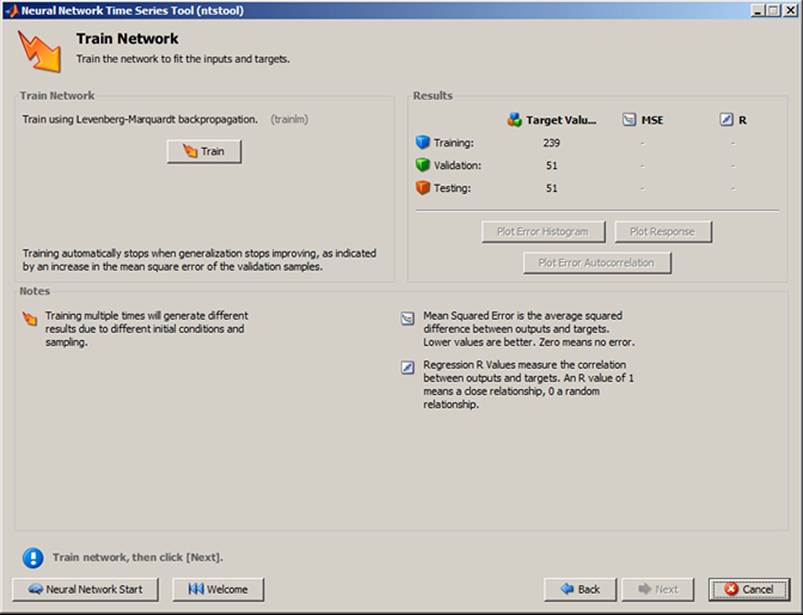
The command Next enables the setup of the network architecture represented by Number of Hidden Neurons and Number of Delays. The default value can be used or it could be changed (see Figure 26). The commands Next and Train start training the neural network (see Figure 27).
The process of training is displayed in the window and after the process of training it is possible to evaluate the graph to determine whether the correct training was done, for example Performance (see Figure 28). It is possible to evaluate the mean square error MSE and fit of prediction (see Figure 29). The process of training may be repeated several times using the command Retrain.
Figure 22. Choice of neural network
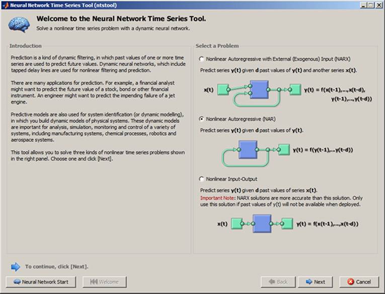
Figure 23. Download of data
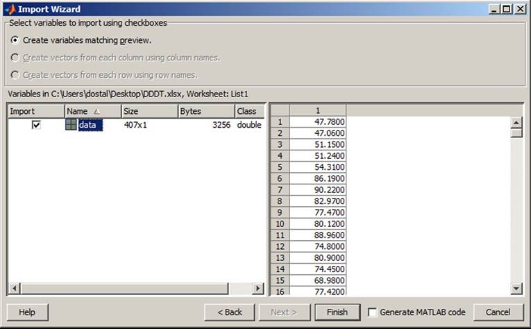
Figure 24. Select of data
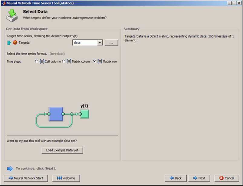
Figure 25. Setup of parameters
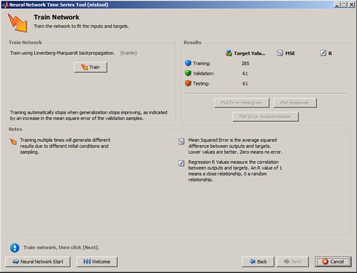
Figure 26. Set of network
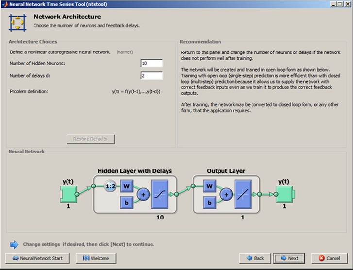
Figure 27. Process of training
When the results of training correspond to the required demands, the output has to be saved as a variable, for example output (see Figure 30).
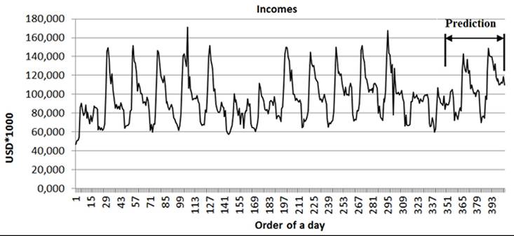
S aved data sets could be used for evaluation, for example to display them at workplace or transferring data into MS Excel. The graph is presented in Figure 31. The graph presents history of 120 days of selling products and its prediction for next 30 days to help to set up a plan of production.
The script could be saved any time in an M-file using the menu Advanced Script shown in Prog. 3.2 in the Appendix.
The advantage of neural network theory for prediction is in their abilities of description of nonlinear economic and financial time series. The disadvantage is, that neural network is like a black box. The prediction of time series fails when time series have a random course.
4. GENETIC ALGORITHMS
4.1 Principles of Genetic Algorithms
Genetic algorithms are used in studies where exact solution by systematic searching would be extremely slow, which is well suited for solving complicated problems. Genetic processes in nature were discovered in the nineteenth century by Mendel and developed by Darwin. The computer realization of genetic algorithms discovered in the 1970s, is connected with the names of J. Holland and Goldberg. Recently there has been considerable expansion of genetic algorithms in the spheres of economic applications and the decision making of firms and companies.
Let us mention a few terms that are used in the branch of genetics: chromosomes, selection,
Figure 28. The process of training
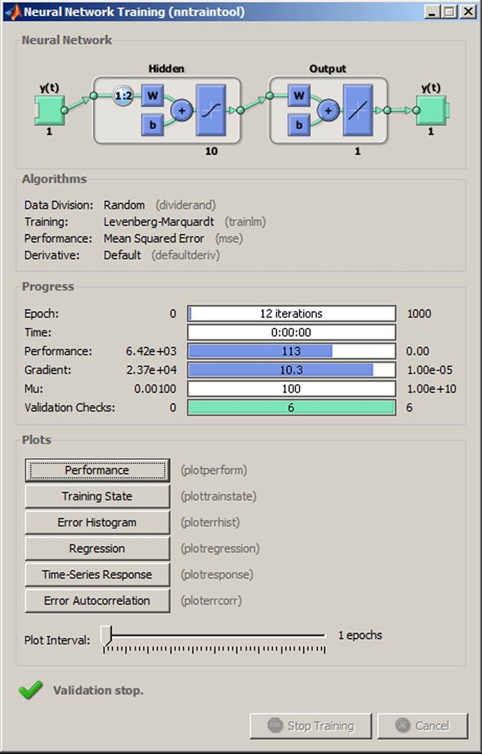
Figure 29. Process of retraining
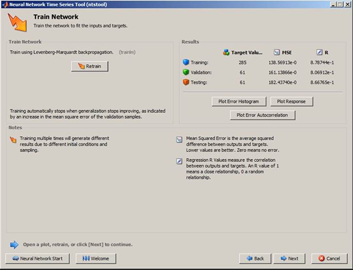
Figure 30. Saving the data
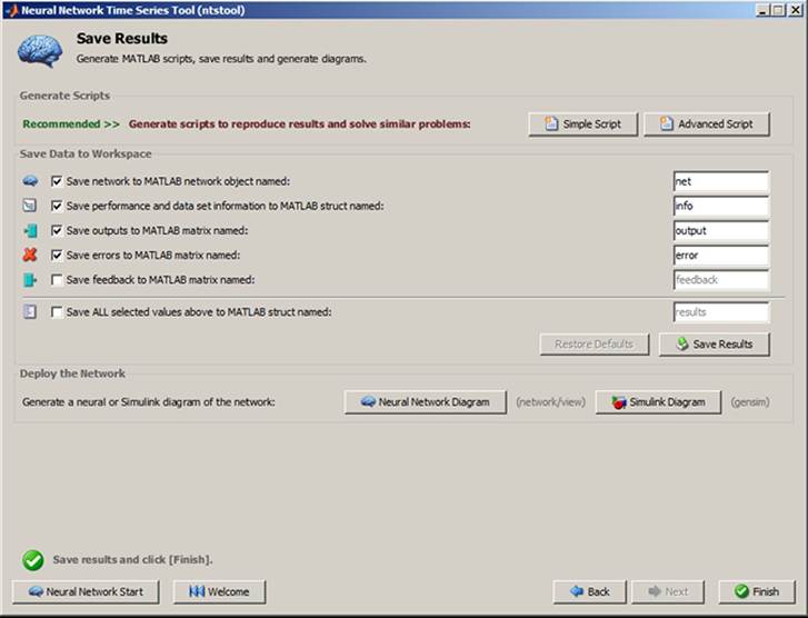
Figure 31. Historical and predicted data of time series
crossover, mutation, population, parents, and offspring. The chromosomes consist of genes (bits). Every gene inherits one or several bits and its position in chromosomes. We say that the chromosomes have locus. The information coded in chromosomes consists of phenotypes. Most of the implementations of genetic algorithm work with the original representation of chromosomes is binary representation: 0 and 1. A chromosome is represented by a binary string, e.g. 0101. These binary strings mostly represent coded decimal numbers. The operators of selection, crossover, and mutation are most often used in genetic algorithms. The diagram is then chained, where the permitted symbol occurs in at least one position (in case of binary representation it is 0 or 1). For the handling of chromosomes, several genetic operators have been proposed. The most used operators are selection, crossover, and mutation.
The process of selection involves the choice of chromosomes that become parents. The fitness of the parents plays an important role in the process of selection. The process of selection is presented in Table 4 when the number 7 (binary 0111) is bigger than 2 (binary 0010). In this case the chromosome with number 7 (binary 0111) progresses to the next generation as the strongest specimen (it leads in computations to better solutions and thus to higher profit).
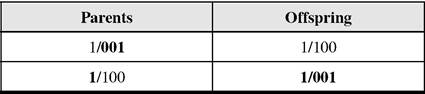
The process of crossover involves the exchange of part of two or more parent’s chromosomes, which causes the modification of the chromosomes of the offspring. The crossover is presented in Table 5.
The crossover can be improved by selection of more parents. The crossover can have more crossing points. This process is called a multi-point cross when more division points are generated. The generalized crossover is done according to the pattern of zeros and ones generated by alternative divisions.
The process of mutation involves the modification of chromosomes. The modification is done
Table 4. Selection
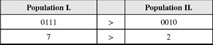
Table 5. Crossover
by random change of some bit. The mutation is not frequent. The mutation is presented in Table 6.
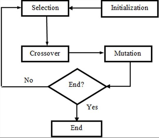
The genetic algorithms work in such a way that the population of chromosomes is created at first. Then the population is changed by means of genetic operators until it is found that the parents are the same (the value of fitness function does not change after some number of iterations). The process of reproduction repeats. Each epoch of population (one generation) represents three steps: selection, crossover, and mutation (see Figure 32).
Note: A fitness function is a function that prescribes the optimality of a solution and correlates closely with the algorithm’s goal (for example maximum profit or minimum costs in business.)
When the genetic algorithm is applied to a problem in the decision making of firms (whose decisions are not reversible), each chromosome codes some solution of the problem (thus a chromo
Table 6. Mutation

some is a genotype and the corresponding solution is a phenotype). Chromosomes with higher fitness functions in genetic algorithms are preferred. The higher the value of the fitness function during the process of iteration, the better the solution of the economic problem. The commercially sold programs do not demand knowledge of binary algebra.
For processes where optimization is required, it is possible to use not only genetic algorithms but also ant colony, particle swarms, bee hive colony algorithms, and others.
The chapter is focused on applications. The genetic algorithm theory is described in books such as (Davis 1991), (Dostal 2011), (Chen et al. 2005), (The MathWorks 2010d).
4.2 Applications of Genetic Algorithms
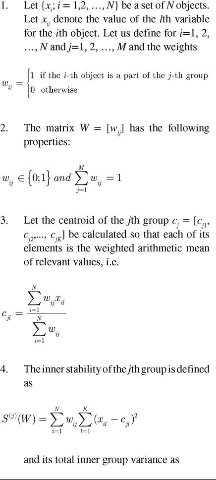
Example 4.1: Cluster analysis problems can be solved by means of genetic algorithms to solve economic problems. The aim of a genetic algorithm as an optimization task is to divide a set of N existing objects into M groups. Each object is characterized by the values of K variables of a K-dimensional vector. The aim is to divide the objects into groups so that the variability inside groups is minimized. The sequence of steps is as follows:
Figure 32. The reproduction process
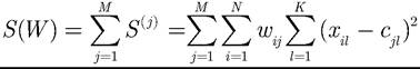
5. The distances between an object and a centroid can be calculated in this case by means of common Euclidean distances
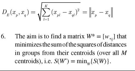
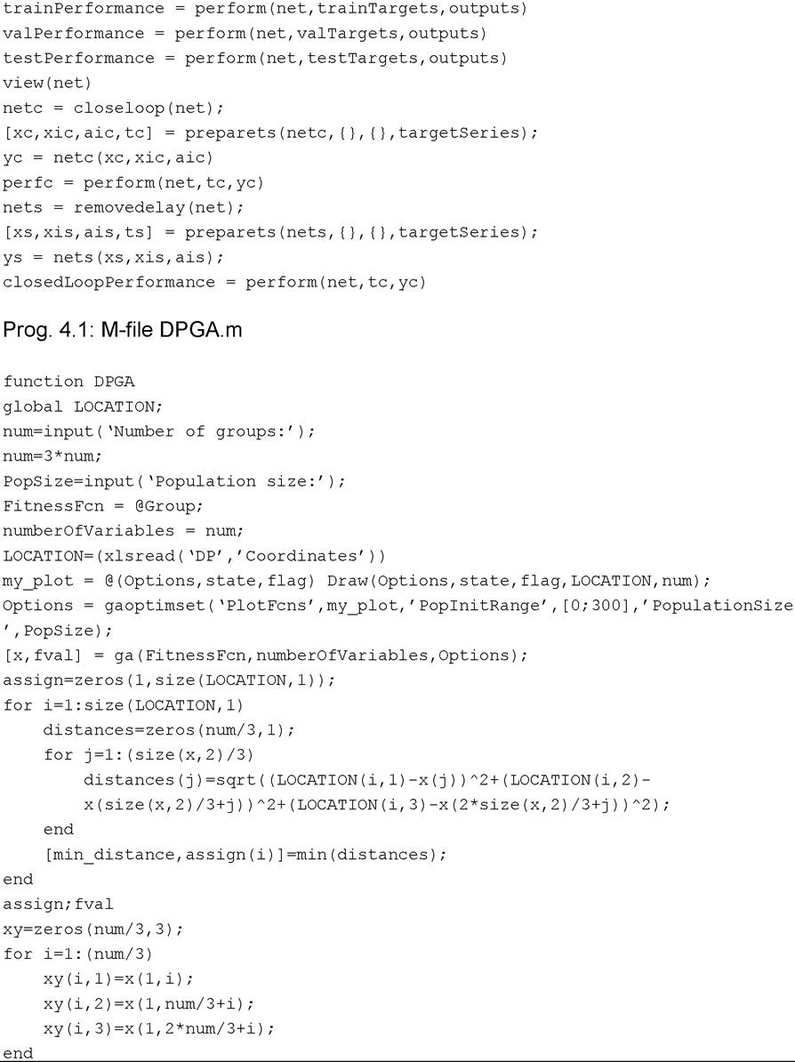
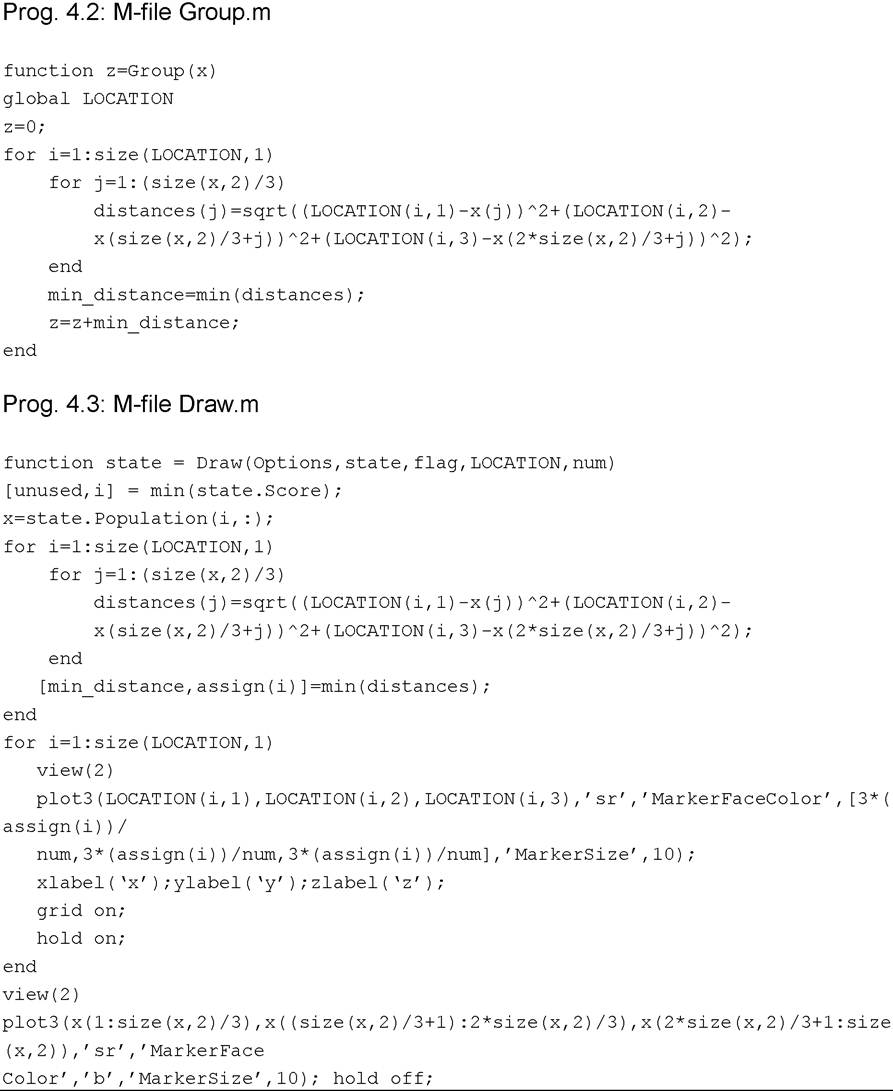
It is convenient to program the task as shown in the program called DPGA.m (Prog. 4.1 ) in the Appendix. The input data are in an MS Excel format file DP.xls which corresponds to Table 7. The Program Group.m (Prog. 4.2 in the Appendix), is used for calculation of Euclidean distances and Program Draw.m (Prog. 4.3 in the Appendix), is used for drawing the graph.
The program enables setting up the number of required groups and the population size. The larger the number of individuals the more precise the solution but the longer the duration of the calculation. Next, the program sets up the options for optimization and the optimization command ga is called. The program involves the calculation of the fitness function and fills the variables with data that inform us about the coordinates of centroids and the assignment of objects to groups and display them. Two- (z axis is zero) or threedimensional tasks can be solved.
The program is started by the command DPGA in MATLAB. Then it is necessary to set up the requested number of groups, e.g. Number of groups
Table 7. Coordinates of places
| Town | xι | X2 | |
| 1 | Prague | 37 | 72 |
| 2 | Brno | 72 | 30 |
| 3 | Ostrava | 100 | 57 |
| 4 | Plzen | 18 | 60 |
| 5 | Olomouc | 83 | 42 |
| 6 | Liberec | 47 | 100 |
| 7 | Hradec Kralove | 59 | 76 |
| 8 | Ceske Budejovice | 36 | 24 |
| 9 | Usti nad Labem | 30 | 99 |
| 10 | Pardubice | 64 | 67 |
| 11 | Zlin | 89 | 32 |
| 12 | Kladno | 90 | 74 |
| 13 | Opava | 94 | 59 |
| 14 | Karlovy Vary | 8 | 81 |
| 15 | Jihlava | 54 | 42 |
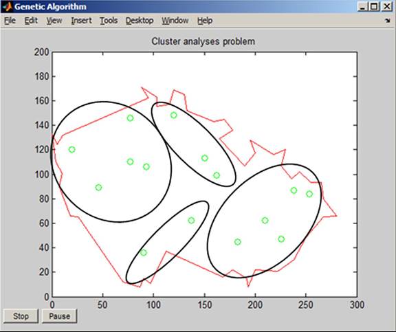
= 4 and Population size = 1000. When the calculation is terminated, the input parameters and results of calculation are displayed on the screen. The results are presented by coordinates of centroids and assignment of places to groups (Results 4.1 in the Appendix). Figure 33 presents the graph and Figure 34 its application in a geographical map.
The advantage of genetic algorithm theory is that enables to solve practical application that belongs to hard difficult problems to solve. The genetic algorithms outperformed classical methods in speed of calculation to find one of the best solutions.
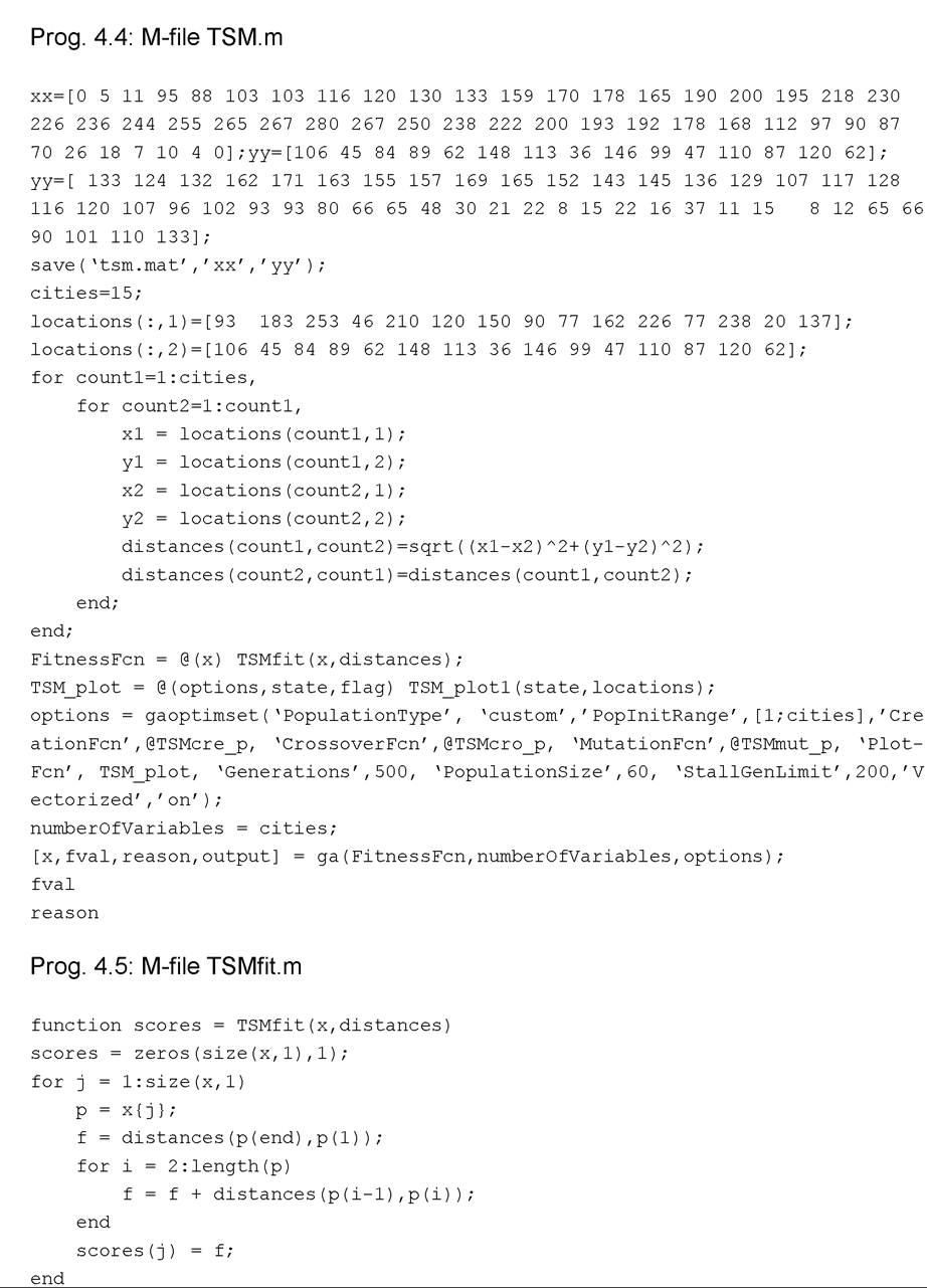
Example 4.2: This example shows that the program environment MATLAB with the Global Optimization Toolbox may also be used to solve the travelling salesman problem. The coordinates of the visited towns x and y must be set up. The aim of the task is to find the shortest tour under the condition of visiting each town only once. The challenge is that when the number of towns is high it is not possible to use exhaustive algorithms to search all combinations. The use of genetic algorithms shortens the calculation time. It finds one of the best solutions very quickly. The problem is programmed in the MATLAB environment (Prog. 4.4 in the Appendix).
The variables xx and yy are the coordinates of contour of Czech Republic. The command save saves the coordinates of contour. The number of cities is set up to 15. The variable locations is setup by coordinates of towns. Next two commands for closed using the command end create two cycles that calculate the distances between each pair of towns. The setup of vectors of pairs of towns x1, y1 and x y2 are saved to variable distances and the distances between towns are calculated by the Pythagorean Theorem as the hypotenuse of coordinates of two points. The cycles fill up only lower left matrix; the next command does this for the upper right one. Thus the cross matrix of distances among towns is set up. The last commands solve the optimization. The program calculates the fitness function FitnessFcn, defined
Figure 33. Places and their centroids
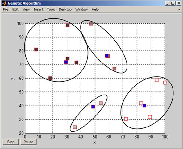
Figure 34. Geographical map
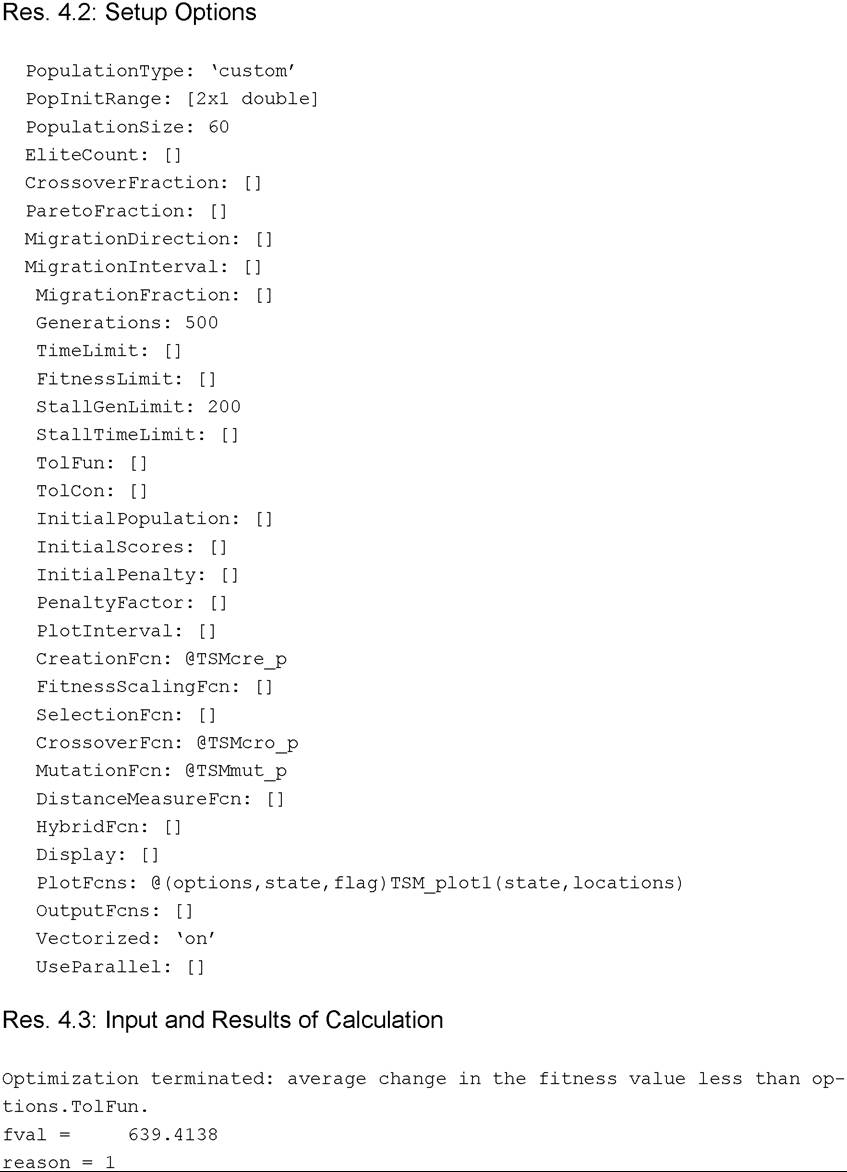
by the M-file as a function called TSMfit(x, distances), with parameters of the number of towns and distances between towns. The resulting value of the function is the total tour distance around the towns for the searched combination. The function TSM_plot1 is placed in the M-file with name M_plot1(state,locations) with parameters options, state a flag. The command gaoptimset sets up variable option obtaining parameters of calculation of optimization by means of the genetic algorithms. It is necessary to do the setup if the default values are not used. The type of population PopulationType is set up as custom; the range PopInitRange as the dimension [1;cit- ies]; the population function CreationFcn as @ TSMcre _p; the crossover function CrossoverFcn as @TSMcro_p; the mutation function MutationFcn as @TSMmut_p; the drawing function PlotFcn as TSM_plot; the number of generations Generation as value 500; the population size PopulationSize as value 60; the termination of the calculation after constancy of 200 generations as StallGenLimit; and the fact that the calculation of fitness function will be done by vector and that the value Vectorized is set up as on.
The next-to-last command sets up the variable numberOfVariables as the number of generated towns. The last command provides the optimization. The key command is ga with the parameters of the fitness function FitnessFcn, number of towns numberOfVariables, and the setup parameters of optimization options. The output variable x is a vector of command of visited towns; fval is a value of the fitness function pepresented by the value of the shortest tour fulfilling the conditions; the value reason provides information about program termination; and the variable output provides information about the calculation of each generation.
Writing out the variable options presents the setup of the parameters of optimization (Results 4.2 in the Appendix). The function TSMfit is defined by an M-file (Prog. 4.5 in the Appendix).
The command zeros sets up the variable scores to be zero. Two cycle commands for closed by commands end provide the calculation of the total tour for the given combination using the cross table distances of distances between towns. The command size returns the values of dimension of matrix in the size m ? n. The command length returns the value of the greatest dimension. The function TSM_plot1 is defined by an M-file (Prog. 4.6 in the Appendix).
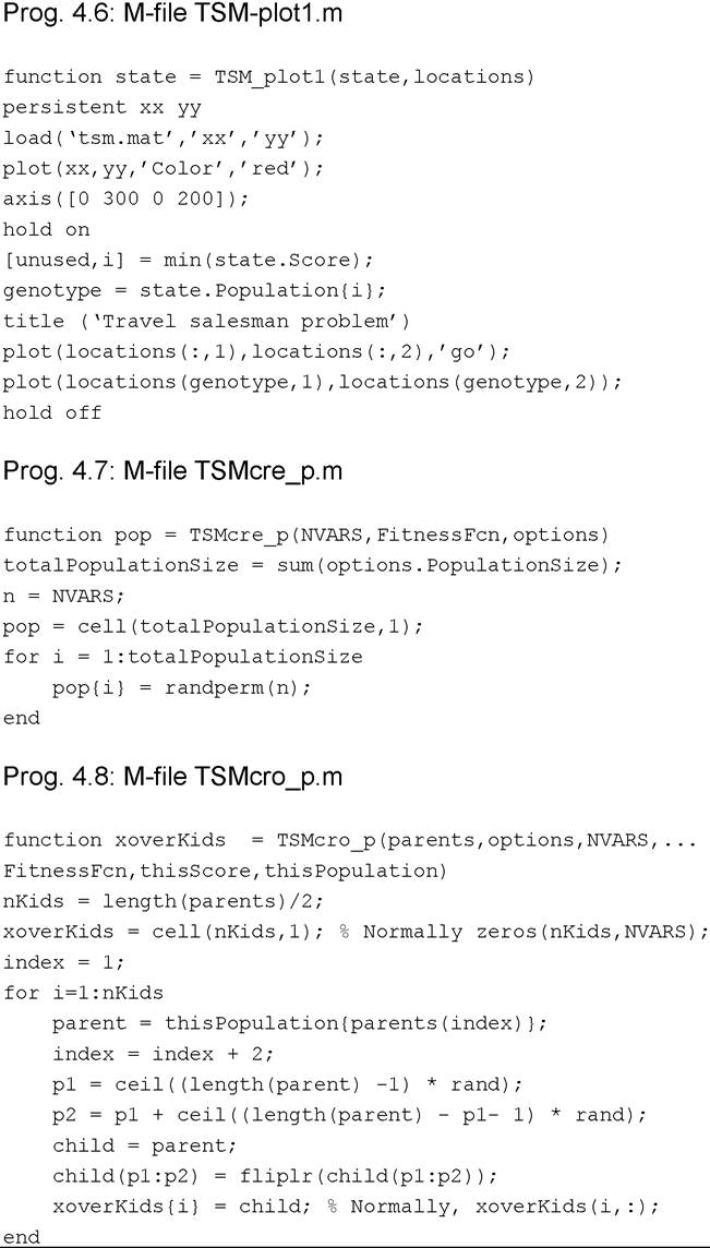
The command persistent ensures that the named variables are local. The command load downloads from tsm. mat file the coordinates of the polygon x, and y that were saved by the TSM.m program. The command plot draws the contour of the state in red colour Color, red. The command axis defines the coordinates of the graph [0 300 0 200] and the command hold on enables the drawing of the actual graph. The next commands set up the values for drawing the towns and their connections. The command min finds the smallest value of the matrix. The command title writes out the title of the graph. The command plot draws the coordinates of towns in a green colour and the next command plot draws connections among towns by a blue line. The command holds off ends the drawing in an active window.
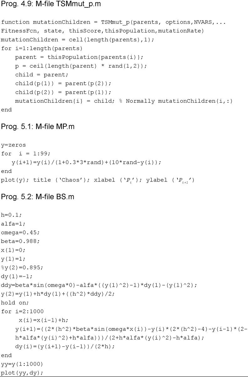
The program uses the M-files for permutation (TSMcre_p), crossover (TSMcro_p), and mutation TSMmut_p that are part of the MATLAB library (Prog. 4.7, Prog. 4.8, and Prog. 4.9 in the Appendix). These M-files are described in the MATLAB library.
The program starts by writing TSM on the display and press the command Enter. The graph is continuously displayed during the process of optimization. Figure 35 presents the graph at the beginning of optimization and Figure 36 at the end of optimization. The shortest tour is found. The mentioned example should be automated as a part of a decision-making tool not dependent on human beings.
The display on the screen presents the end of optimization, the value of the fitness function, and the reason for the end of the calculation (Results 4.3 in the Appendix).
Figure 35. Tour before optimization
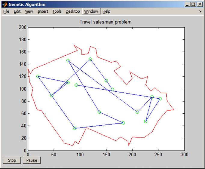
Figure 36. Tour after optimization
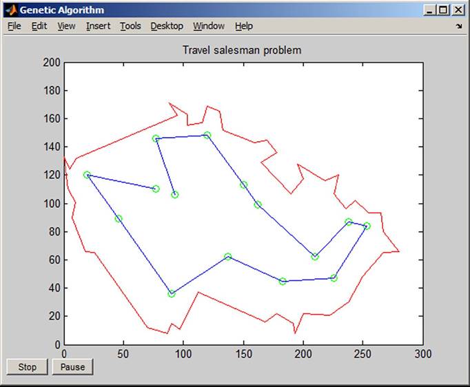
The advantage of using the genetic algorithm is in the speed of calculation, especially with increasing numbers of visited towns. Note: It is empirically proved and described in the literature that the genetic algorithms found the suboptimum near to the global optimum successfully and very quickly.
Example 4.3: The optimization task could be solved by various methods, not only by genetic algorithms that are quite often used in business and public services. Some algorithms can give better solutions than others. Different results are obtained when the entire state space of solutions is not searched. For example the Exhaustive method finds the best solution, but the calculations could last weeks. The present example compares twelve methods solving the travelling salesman problem (Exhausive, Backtracking, RandomSearch, Greedy, Hill Climbing, Simulated Annealing, Tabu Search, Ant Colony, Genetic Search, Particle Swarms, DNA Genetic Search, and Bee Hive Colony). Ten places were used and it was measured the time of calculation, the value of fitness function, and number of attempts that were necessary for finding the minimum value, which in this case is Yes (Table 8).
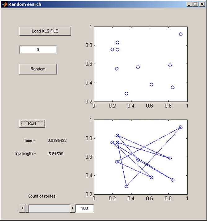
The best results from the point of view of fitness function, speed of calculation, and number of attempts were obtained using the Greedy, Ant Colony, and Bee Hive Colony algorithms. Good results were provided by Tabu Search, Particle Swarms, and DNA Genetic Search. The Random Search and Simulated Annealing algorithm found the longest tours, which mean undesirable high expenses of the tour. The Exhaustive algorithm search had the highest calculation time, but it found the global minimum for this problem.
Figure 37 presents the best solution of the optimization task when the whole state space of solution was searched by the Exhaustive algorithm. The worst time of calculation and the worst solution were obtained using Random Search, with results not usable in practice (Figure 38).
We should mention that the optimization processes have their pros and cons. Their virtues include the fact that they solve complicated problems very easily and search for the maximum or minimum very successfully. The Genetic algorithm, Ant Colony, Particle Swarm, and Bee Hive Colony, in comparison with classical searching algorithms, search for the local extreme better (finding the solution nearest to the optimum) and require fewer math operations than the other methods. Evolution algorithms are useful for the solution of various problems that must be solved in decision making in business, economics, and finance.
Optimization methods based on evolutionary algorithms solves successfully difficult problems such as travel salesman problem, especially with increasing number of cities. Some methods give better results and some give worse results. The use of various methods must be tested and the best one to be use in practice.
5. THEORY OF CHAOS
5.1 Fundamentals of Chaos
An early proponent of chaos theory was Henri Poincare. In the 1880s, while studying the three-body problem, he found that there can be orbits which are nonperiodic, and yet not forever increasing nor approaching a fixed point. Later studies, also on the topic of nonlinear differential equations, were carried out by G.D. Birkhoff and A. N. Kolmogorov. An early pioneer of the theory was Edward Lorenz whose interest in chaos came about accidentally through his work on weather prediction in 1961. Lorenz’s discovery, which gave its name to Lorenz attractors, showed that even detailed atmospheric modelling cannot in general make long-term weather predictions. Mandelbrot described both the “Noah effect” and the “Joseph effect.” In 1975 Mandelbrot published The Fractal Geometry of Nature, which became a classic of chaos theory. The same year, James Gleick published Chaos: Making a New Science, which
Table 8. The comparison of optimization methods
| Method | Time [sec] | Fit. F. | No. of Attempts | Min |
| 1. Exhaustive | 426.21405 | 2.6274 | 1x | Y |
| 2. Back Tracking | 21.54944 | 2.6274 | 1x | Y |
| 3. Random Search | 0.01945 | 3.43841 | 20x | N |
| 4. Greedy | 0.02030 | 2.6274 | 1x | Y |
| 5. Hill Climbing | 0.00543 | 2.6274 | 10x | Y |
| 6. Simulated Annealing | 0.01638 | 2.91421 | 20x | N |
| 7. Tabu Search | 0.38592 | 2.6272 | 2x | Y |
| 8. Ant Colony | 1.0983 | 2.6274 | 1x | Y |
| 9. Genetic Search | 1.33721 | 2.65847 | 5x | Y |
| 10. Particle Swarms | 1.75342 | 2.62739 | 3x | Y |
| 11. DNA Genetic Search | 21.1449 | 2.62739 | 3x | Y |
| 12. Bee Hive Colony | 0.02345 | 2.674 | 1x | Y |
Figure 37. Graph from exhaustive methods
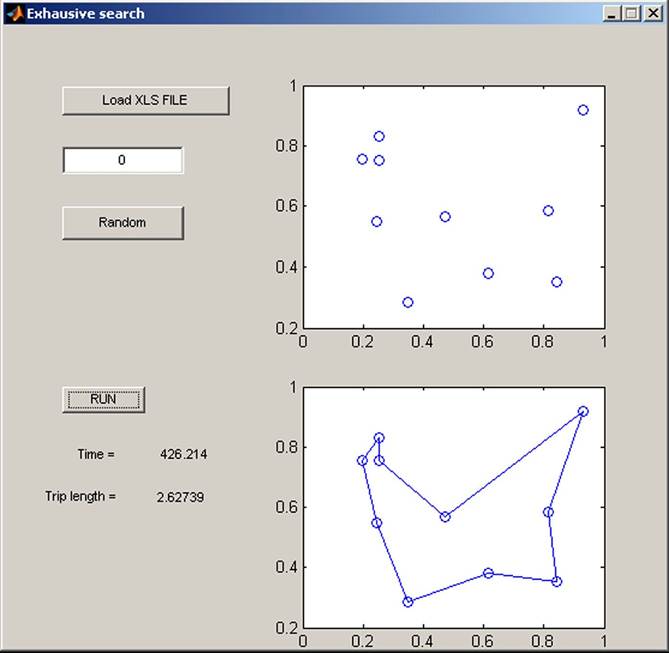
Figure 38. Graph from random search methods
became a best-seller and introduced the general principles of chaos theory.
The theory of chaos came into being in solution of technical problems, where it describes the behaviour of nonlinear systems that have some hidden order, but still behave like systems controlled by chance. A linear model can describe a real system only if it is linear. If this is not fulfilled, then such models can simulate the real system only under ideal conditions, only for a short time. If a system is a nonlinear dynamic, a deterministic system it can generate not only the permanent trends and cycles, but it can also include random-looking behaviour. Processes of such behaviour are present in the economy.
In this respect we can talk about two categories that are in opposition to each other: order and randomness. Chaos is something in between. It involves some degree of order. Some phenomena can appear random, but after the study of these phenomena some inner order can be discovered that governs these phenomena. For example, the movement of people at a railway station can appear accidental, but in fact it is behaviour with order controlled by the arrival and departure of trains. Also, the economy can exist in states of various degrees of order, chaos, and randomness. The behaviour of an economy is influenced quite often by natural disasters, political changes, etc.
In connection with chaos it is possible to speak about a so-called attractor, which represents an equilibrium position. An attractor is a condition towards which a dynamical system evolves over time. That is, points that get close enough to the attractor remain close even if slightly disturbed. Geometrically, an attractor can be a point, a curve, or even a complicated set with a fractal structure known as a chaotic attractor.
The geometrical explanation of an attractor could be done with the help of a pendulum. The attractor can be:
• Point: The stability is represented geometrically by a point. For example, when a pendulum is displaced, its final equilibrium position is reached when movement ceases.
• Cycle: The balance is represented geometrically by a limited cycle. For example, when a pendulum is moving with constant energy (potential energy plus kinetic energy = const.), its equilibrium position is reached when movement is cyclical.
• Chaotic: It is represented geometrically by order underlying the apparent chaos. For example, when the pendulum is driven by random energy, then the equilibrium position will be represented by a movement in zone (no point or cycle).
The chapter is focused on applications. The chaos theory is described in books such as (Barnsley 1993), (Dostal 2011), (Gleick 1996), (Peters 1994), (Peters 1996), (Trippi 1995), (The MathWorks 2010a).
5.1 Applications of Chaos
Example 5.1: The complicated behaviour in economy could be illustrated by the equation in the form
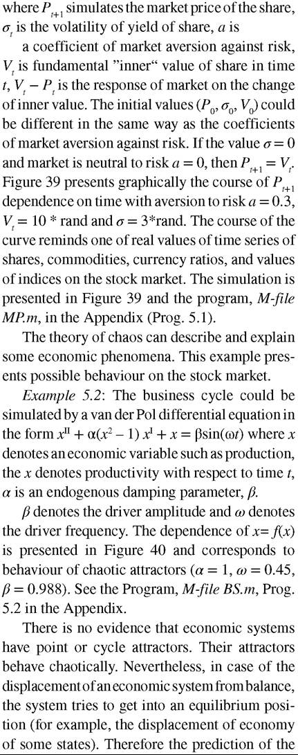
Figure 39. The graph of function Pt+1 with parameter a = 0.3
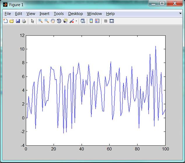
Figure 40. Graph of chaotic attractor
behaviour of economic development is restricted by contemporary knowledge, and the longer range predictions are uncertain. The theory of chaos could describe some economic and financial phenomena. The research is done very intensively.
FUTURE RESEARCH DIRECTIONS
The use of soft computing finds its place in the field of business, economics, and finance among other methods. It is done by successful applications in practice where especially vague terms, uncertainty imprecision, uncertainty, vagueness, semi-truth, approximations and non-linear behaviour with noise are frequent phenomena. The future research must be directed to build-up the models for complex decision making processes. The future trends that are expected from the soft computing technologies, which may satisfy these needs, are as follows: new fuzzy, neural networks, genetic algorithms models and their combinations. The future research will be focused in various applications to support decision making to be quicker and more precise because processed amount of data are increasing exponentially. More and more decision making will be done by automatic systems without influence of human being. These automatic decision systems must be designed to be robust and avoiding failures.
The future research of soft computing applications in business, economics, and finance will be focussed especially on improvement in these fields: data mining, data analyses, mortgage loan applications, loan pre-screening processes, client financial risk, client asset allocation, marketing, manufacturing at economic optimum, searching for faulty or fraudulent audits or suspicious financial transactions, predictive optimal supply-chain, predictive intelligent security, protection credit card fraud, time forecasting, time series prediction, prediction of thrift failures, new product pricing, customer classification, investment management and risk control, investment advising, detection of financial crisis, flow shop scheduling, solution of travelling salesman problem, etc.
The development of quick, more precise, parttime or fully automated decision making systems where soft computing methods will be used they will save time, decrease wrong decisions, avoiding human failures, reduce costs that can lead to higher profit, or decrease expenses in business and they can help to compete successfully.
CONCLUSION
The business, economic and financial applications have specific features in comparison with others. The processes are focused on optimizing income or profit, or decreasing expenses. Therefore, such applications, both successful and unsuccessful, are not published very often because of secrecy in the highly competitive environments among firms and institutions. The advanced decision methods can help in decentralization of decision-making processes to become standardized, reproduced, and documented. The advanced decision-making methods play very important roles in companies because they help to reduce costs that can lead to higher profit and they can help to compete successfully, or decrease expenses in institutions. The decision-making processes in business are very complicated because they include political, social, psychological, economic, financial, and other factors. Many variables are difficult to measure; they may be characterized by imprecision, uncertainty, vagueness, semi-truth, approximations, and so forth.
The use of the theories mentioned above is in the sphere of analyses and simulation. Except the applications such as risk investment, risk management, optimization, prediction of time series, journey optimization, description of phenomena it could be many other applications it could be mentioned mortgage loan risk evaluation, direct mailing decision making, stock market decision, stock trading decision, decision making evaluation, client risk evaluation, supplier risk evaluation, etc.
The use of these computing methods can lead to higher quality of analyses and simulations that can be used for decision-making and control processes in business, economy, financial areas, or the public sector.
REFERENCES
Aliev, A., & Aliev, R. (2002). Soft computing and its applications. World Scientific Publishing.
Altroc, C. (1996). Fuzzy logic & neurofuzzy applications in business & finance. USA: Prentice Hall.
Azoff, E. M. (1994). Neural network time series forecasting of financial markets. USA: John Wiley.
Barnsley, M. F. (1993). Fractals everywhere. USA: Academic Press Professional.
Bose, K., & Liang, P. (1996). Neural networks, fundamentals with graphs, algorithms and applications. USA: McGraw-Hill.
Chen, G. (2000). Controlling chaos and bifurcations in engineering systems. China: CRC Press.
Chen, P., Jain, L., & Tai, C. (2005). Computational economics: A perspective from computational intelligence. Hershey, PA: Idea Group Publishing. doi:10.4018/978-1-59140-649-5
Chen, S., Wang, P., & Wen, T. (2004). Computational intelligence in economics and finance. New York, NY: Springer.
Chen, S., Wang, P., & Wen, T. (2007). Computational intelligence in economics and finance (Vol. II). New York, NY: Springer. doi:10.1007/978- 3-540-72821-4
Davis, L. (1991). Handbook of genetic algorithms. USA: Int. Thomson Com. Press.
Dostal, P. (2008). Advanced economic analyses. Brno, Czech Republic: VUT - FP.
Dostal, P. (2011). Advanced decision making in business and public services. Brno, Czech Republic: CERM.
Ehlers, F. J. (2004). Cybernetic analysis for stock and futures. USA: John Wiley.
Franses, P. H. (2001). Time series modelsfor business and economic forecasting. UK: Cambridge University Press.
Gately, E. (1996). Neural networks for financial forecasting. USA: John Wiley.
Gleick, J. (1996). Chaos. USA: Ando Publishing.
Hagan, T., & Demuth, B. (1996). Neural network design. USA: PWS Publishing.
Hanselman, D., & Littlefield, B. (2005). Mastering MATLAB 7. USA: Prentice Hall.
Kazabov, K., & Kozma, R. (1998). Neuro-fuzzy techniques for intelligent information systems. Germany: Physica-Verlag.
Klir, G. J., & Yuan, B. (1995). Fuzzy sets and fuzzy logic, theory and applications. New Jersey, USA: Prentice Hall.
Li, Z., Halong, W. A., & Chen, G. (2006). Integration of fuzzy logic and chaos theory. New York, NY: Springer. doi:10.1007/3-540-32502-6
Peters, E. E. (1994). Fractal market analysis-Applying chaos theory to investment & economics. USA: John Wiley.
Peters, E. E. (1996). Chaos and order in the capital markets: A new view of cycles, prices. USA: Wiley Finance Edition.
The MathWorks. (2010a). MATLAB - User’s guide. The MathWorks.
The MathWorks. (2010b). MATLAB - Fuzzy logic toolbox - User’s guide. The MathWorks.
The MathWorks. (2010c). MATLAB - Neural network toolbox - User’s guide. The MathWorks. The MathWorks. (2010d). MATLAB - Global optimization toolbox - User ,s guide. The MathWorks.
Trippi, R. R. (1995). Chaos & nonlinear dynamics in the financial markets. USA: Irwin Professional Publishing.
ADDITIONAL READING
Ahn, H., Kyoung, K., & Han, I. (2006). Hybrid genetic algorithms and case-based reasoning systems for customer classification. Expert Systems: International Journal of Knowledge Engineering and Neural Networks, 23(3), 127-144. doi:10.1111/j.1468-0394.2006.00329.x
Bernice, C. (1997). The edge of chaos-Financial booms, bubbles, crashes and chaos. UK: John Wiley.
Bojadziev, G., & Bojadziev, M. (2007). Fuzzy logic for business, finance, and management, 2nd ed. World Scientific Publishing Co. Pte. Ltd.
Chian, A., Borotto, F. A., Rempel, E. L., & Rogers, C. (2005). Attractor merging crisis in chaotic business cycles. Chaos, Solitons, and Fractals, 24(3), 869-875. doi:10.1016/j.chaos.2004.09.080
Comunale, Ch., Rosner, R., & Sexton, T. (2010). The auditor’s assessment of fraud risk: A fuzzy logic approach. Journal of Forensic & Investigative Accounting, 3(1), 149-194.
Delgado, M. C. Pegalajar, M. C., Cuellar, & M. P. (2006). Memetic evolutionary training for recurrent neural networks: An application to timeseries prediction. Expert Systems: International Journal of Knowledge Engineering and Neural Networks, 23(2), 99-115. doi:10.1111/j.1468- 0394.2006.00327.x
Feng, S., Xu, L., Tang, C., & Yang, S. (2003). An intelligent agent with layered architecture for operating systems resource management. Expert Systems: International Journal of Knowledge Engineering and Neural Networks, 20(4), 171-178. doi:10.1111/1468-0394.00241
Hamad, A., Sanugi, B., & Salleh, S. (2011). Neural network and scheduling: Neural network and job scheduling problems. Lambert Academic Publishing.
Hand, D., & Mannila, H. (2001). Principles of data mining. USA: The MIT Press.
Herbst, F. (1992). Analysing and forecasting futures prices. USA: John Wiley.
Jiao, J., & Zhang, Y. (2010). Product portfolio identification based on association rule mining. CAD Computer Aided Design, 37(2), 149-172. doi:10.1016/j.cad.2004.05.006
Joo, K. O., Kim, T. Y., & Kim, C. (2006). An early warning system for detection of financial crisis using financial market volatility. Expert Systems: International Journal of Knowledge Engineering and Neural Networks, 23(2), 83-98. doi:10.1111/j.1468-0394.2006.00326.x
Joseph, K., Wintoki, M., & Zhang, Z. (2011). Forecasting abnormal stock returns and trading volume using investor sentiment: Evidence from online search. International Journal of Forecasting, 27, 116-1127. doi:10.1016/j.ijforecast.2010.11.001
Kuo, I., Shi-Jinn Horng, S., Kao, T., Lin, S., Lee, C., Chen, Y., & Terano, T. (2010). A hybrid swarm intelligence algorithm for the travelling salesman problem. Expert Systems: International Journal of Knowledge Engineering and Neural Networks, 27(3), 166-179. doi:10.1111/j.1468- 0394.2010.00517.x
Li, E. Y. (1994). Artificial neural networks and their business applications. Information & Management, 27(5), 303-313. doi:10.1016/0378- 7206(94)90024-8
Liebowitz, J., Krishnamurthy, V., Rodens, I., Houston, C., Baek, S., Liebowitz, A., & Potter, W. (1997). Intelligent scheduling with generically used expert scheduling system: Development and testing results. Expert Systems: International Journal of Knowledge Engineering and Neural Networks, 14(3), 119-128. doi:10.1111/1468- 0394.00048
Liebowitz, J., Rodens, I., Zeide, J., & Suen, C. (2000). Developing a neural network approach for intelligent scheduling in generically used expert scheduling system. Expert Systems: International Journal of Knowledge Engineering and Neural Networks, 17(4), 185-190. doi:10.1111/1468- 0394.00140
Manolas, D. A., Efthimeros, G. A., & Tsahalis,
D. T. (2001). Available technologies and their optimal operating conditions for the process industry. Expert Systems: International Journal of Knowledge Engineering and Neural Networks, 18(3), 124-130. doi:10.1111/1468-0394.00165
Nikolopoulos, C., & Fellrath, P. (1994). A hybrid expert system for investment advising. Expert Systems: International Journal of Knowledge Engineering and Neural Networks, 11(4), 245-250. doi:10.1111/j.1468-0394.1994.tb00332.x
Rud, O. (2001). Data mining cookbook: Modeling datafor marketing, risk and customer relationship management. USA: John Wiley.
Trif, S. (2011). Using genetic algorithms in secured business intelligence mobile applications. Informatica Economica, 15(1).
Tsai, C., Tsai, Ch. W., & Tseng, C. (2003). A new and efficient ant-based heuristic method for solving the traveling salesman problem. Expert Systems: International Journal of Knowledge Engineering and Neural Networks, 20(4), 179-186. doi:10.1111/1468-0394.00242
Wang, H. (2005). Flexible flow shop scheduling: Optimum, heuristics and artificial intelligence solutions. Expert Systems: International Journal of Knowledge Engineering and Neural Networks, 22(2), 78-85. doi:10.1111/j.1468- 0394.2005.00297.x
Weigend, A. (1993). Time series prediction: Forecasting the future and understanding the past. Massachusetts: Addison-Wesley.
Wong, B., Bodnovich, K., & Selvi, Y. (1994). A bibliography of neural network business applications research. Expert Systems: International Journal of Knowledge Engineering and Neural Networks, 12(3), 253-261. doi:10.1111/j.1468-0394.1995. tb00114.x
Yamada, T., & Nakano, R. (1997). Genetic algorithms for job-shop scheduling problems. In Proceedings of Modern Heuristic for Decision Support (pp. 67-81). London: Unicom.
Yu, K., Luo, Z., Chou, C., Chen, C., & Zhou, J. (2007). In T. Enokido (Ed.), A fuzzy neural network based scheduling algorithm for job assignment on computational grids (Vol. 4658, pp. 533-542). Lecture Notes in Computer Science Heidelberg, Germany: Springer. doi: 10.1007/978- 3-540-74573-0_55
Zhang, G. P. (2004). Neural networks in business forecasting. Hershey, PA: Idea Group Publishing.
KEY TERMS AND DEFINITIONS
Artificial Neural Network: A mathematical model or computational model that is inspired by the structure and/or functional aspects of biological neural networks.
Business: The state of being busy either as an individual or society as a whole, doing commercially viable and profitable work.
Economic: Economics is the social science that analyses the production, distribution, and consumption of goods and services.
Finance: The management of money or “funds” management.
Fuzzy Logic: Deals with reasoning that is approximate rather than fixed and exact.
Genetic Algorithm: An evolutionary algorithm-based methodology inspired by biological evolution to find computer programs that perform a user-defined task.
Optimization: The act of rendering optimal.
Soft Computing: Soft computing is a term applied to a field within computer science which is characterized by the use of inexact solutions to computationally-hard tasks.
This work was previously published in Meta-Heuristics Optimization Algorithms in Engineering, Business, Economics, and Finance, edited by Pandian M. Vasant, pages 41-86, copyright 2013 by Information Science Reference (an imprint of IGl Global).
Results