NASH EQUILIBRIUM
The Concept of Nash Equilibrium
The Nash Equilibrium is a concept of game theory in which the optimal outcome of a game is one in which no player has an incentive to deviate from her or his chosen strategy after considering the choices of opponents.
Each competitor is assumed to be rational. There may be a single Nash Equilibrium, double Nash Equilibriums and multiple Nash Equilibriums. Table 1 describes double Nash Equilibriums.The Case of the Maxmin Strategy
This strategy may be derived from the assumption of rationality in the Nash Equilibrium. S ometimes Bank X may behave rationally and expect Bank Y to do the same. Bank X may categorize actions as ‘right’ or ‘wrong’. Bank X may consider lending with due diligence to be the ‘right’ action and lending liberally to the customers having long term banking relationship to be ‘wrong’ because choosing the ‘right’ pays maximum and choosing the ‘wrong’ pays the minimum. However, the RBI established strict rules for the banks lending to the real estate sector (Economic Times, 2011). Bank X expects the considerations for ‘right’ and ‘wrong’ on part of Bank Y to be similar. In Table 2, Bank X gains 2 after choosing ‘right’ whether
Table 1. Additional Profit out of Loan
| Y Bank | |||
| Üî^^ĺňĺĚ-Ĺřĺ-Optian- Free-Loan | High-Interest-Rate-Loan with Foreclosure pttion | ||
| X Bank | 3, 3 | 5, 5 | |
| High-Interest-Rate-Loan with Foreclosure Option | 5, 5 | 3, 3 | |
Table 2. Additional profit out of loan: Maximin Strategy
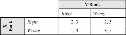
the Y Bank chooses the ‘right’ or the ‘wrong’ and gains more in case Bank Y chooses ‘wrongly’.
However, after choosing ‘right’ or ‘the ‘wrong’ B ank Y gains uniformly irrespective of what B ank X chooses, but Bank Y gains relatively more by choosing ‘wrong’. Though Bank X believes that choosing ‘wrong’ provides minimum gain, in an attempt to maximize the minimum it chooses ‘ wrong ’. The numerical figures in the bottom right cell constitute the Nash Equilibrium.Mixed Strategy
The strategies in Table 1 and Table 2 are called “pure strategy” because a bank chooses only one action, say, either of ‘lending with due diligence’ and ‘lending liberally’ or, either of ‘low-interest- rate-option-free-loan’ and ‘high-interest-rate-loan with foreclosure option’. But, there may be cases in which a bank prefers to choose a mix of both actions. Suppose the banks are operating in the housing loan market where the loan must accompany property insurance. Hence, both the banking product and the property insurance product are sold under the same roof of a bank (e.g., the new generation private sector banks such as ICICI Bank and HDFC Bank assign general insurance business targets including property insurance business to their banking staff and some fast improvising public sector banks like the State Bank of India gives a property insurance agency to some of its banking staff).
In the context of this chapter, it may be assumed that both Bank X and Bank Y sell the housing loan product as well as the property insurance product.
B ank X would obtain maximum advantage if it can sell a property insurance product to a borrower to whom it is going to deliver a housing loan product, but will not object if its borrower buys the property insurance product from Bank Y. The situation is described in Table 3 and Figure 2.
Here both the competitors would prefer the cells - top right and bottom left together. There is no Nash Equilibrium in pure strategies such as Table 1 and Table 2. This is called a “mixed strategy” because the expected additional profit to a bank from each business is the probability- weighted average of two combinations - in one of which the other business is also combined.
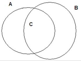
Here, one may explore the probability such as ‘the probability that a customer would choose Bank X out of the two banks for a loan.Here ‘A’ indicates the selling of a housing loan product with or without selling any property insurance product by a bank. ‘B’ means selling a property insurance product with or without selling any housing loan product by a bank. ‘C’ means selling of both products by a bank.
Table 3. Additionalprofit out of loan and/or insurance: Mixed strategy
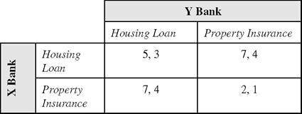
Figure 2. Venn diagram
A Practical Example
If two banks are ready to sanction housing loan for approved projects like Godrej Prakriti, the above game may happen (Commonfloor, 2013).
Axiom I: There is a probability of 0.67 that a customer would approach Bank X for a loan and hence the probability of 1 - 0.67 = 0.33 that a customer would approach Bank Y for the same loan1.
Axiom II: There is a probability of 0.45 that a customer would approach Bank X for a property insurance product and hence the probability of 1-0.45 = 0.55 that he would approach Bank Y for the same2.
Corollary I: The expected additional profit to Bank X from selling a property insurance product is 2.4.
Proof of Corollary I: Here, there are two outcomes in total in the selling of a property insurance product by Bank X: (i) additional profit of ‘7’ from selling of a property insurance product with selling a housing loan product; (ii) additional profit of ‘2’ from selling of a property insurance product without a housing loan product. The probabilities of selling of a housing loan product and a property insurance product by a bank are independent of each other. Hence, the joint probability of selling of a housing loan product and a property insurance product by Bank X equals 0.67 x 0.45 ≈ 0.3 and the probability of selling of a property insurance product without a housing loan product by Bank Y equals 0.45 x 0.33 ≈ 0.15.
The expected additional profit of selling of a property insurance product by Bank X equals (0.3x7) + (0.15 x 2) = 2.4.Corollary II: The expected additional profit to Bank Y from selling a property insurance product is 0.87.
Proofof Corollary II: U sing the logic in Corollary I, one may find that the joint probability of selling of a housing loan product and a property insurance product by Bank Y equals 0.33 x 0.55 ≈ 0.18 and the probability of selling of a housing loan product without a property insurance product by Bank Y equals 0.33 x 0.45 ≈ 0.15. The expected additional profit of selling of a property insurance product by Bank Y equals (0.18x4) + (0.15x1) = 0.87.
Corollary III: The expected additional profit to Bank X from selling a housing loan product is 3.95.
ProofofCorollary III: There are two outcomes in total in the selling of a housing loan product by Bank X:
1. Additional profit of ‘7’ from selling of a property insurance product with a housing loan product;
2. Additional profit of ‘2’ from selling of a housing loan product without property insurance ‘5’.
The joint probability of selling of a housing loan product without selling a property insurance product is 0.67x0.55 ≈ 0.37. The expected additional profit to Bank X from selling a housing loan product is (0.3x7) + (0.37x5) = 3.95.
Corollary IV: The expected additional profit to Bank Y from selling a housing loan product is 1.46.
Proofof Corollary IV: There are two outcomes in the selling of a housing loan product by Bank Y:
1. Additional profit of ‘4’ from selling of a property insurance product with a housing loan product;
2. Additional profit of ‘2’ from selling of a housing loan product without property insurance ‘3’.
The joint probability of selling of a housing loan product without selling a property insurance product by Bank Y is 0.33x0.45 ≈ 0.37. The expected additional profit to Bank Y from selling a housing loan product is 0.18x4 + (0.37x2) = 1.46.
The ‘Tit for Tat' Strategy
In a duopolistic arrangement, the banks in a housing loan market may try to undercut each other by lowering the interest rate. In the first round of the game, the bank setting a lower interest rate than its rival may earn short term profit, but if the game is repeated an infinite number of times, the rival also would do the same and the short run profit may vanish. This is called the ‘Tit for Tat’ Strategy.
The Sequential Game and the Decision Tree
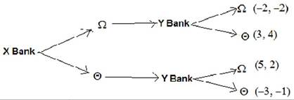
When the two banks are not in collusion, they may assume the other would do its best but itself would benefit if it takes the first move. There are two retail housing loan products on demand - one with a 10% down-payment and a 12% interest rate (let ‘Q’ denote this product) and another with a 15% down-payment and an 8% interest rate (let ‘0’ denote this product). Each product would maximize the profit of only one Bank. Both banks believe that whoever would first introduce one of the above two products would earn more profit from that product than would the other; hence, each bank chooses to respond to the other Bank by launching the other product. If Bank X launches Ω, Bank Y instantly responds by launching Θ. This is called a “sequential game” because of this instant response from the competitor. If it occurs in multiple rounds, the sequences would be similar. This may be explained using the decision tree in Figure 3.
In response to one rival, if the other introduces the same product, both lose. But in response one rival when the other launches its best product both gain. For Bank X, launching Ω first gives maximum profit of ‘5’, whereas for Bank Y launching Θ in response to the action of Bank X provides the maximum profit of ‘3’. A bank decides on its move looking at the pay-off to it in the end of the game. This is called “backward calculation” and this form of the game is called the extensive form of the game (Pindyck & Rubinfeld, 1995, p. 470).
Commitment
The game in Figure 3 reveals that if a bank responds to the move of the other by launching the same product, a loss occurs.
Hence, each bank commits itself to launch the other product in response. Such a commitment by one bank is fruitless unless the other believes it. Therefore, a bank should consider some strategic move such as advertisements in national daily publication which occupies a large space in the front page of the newspaper or in the top rated television channels.Threat
Some actions of one player may work as a threat to the other. If Bank X has already launched product Ω, it is a threat to Bank Y in the case where Bank Y wishes to retain the down-payment at a level of 10% because then Bank Y has no other option to lower interest rate below 12%. If Bank Y charges a rate of interest higher than 12%, it would simply be out of the industry.
Figure 3. Sequential game