THE ISSUES

In the context of the above game, it is interest­ing to discuss the issues raised by the Faculty of Management Economics (2013).

The Issue of Zero-Sum Game

The above game can be a zero-sum when there is no collateral mortgage (i.e., default would benefit the borrower at the lender’s cost and vice versa).

The Issue of Safest Strategy

If each player suspects that other would defect, it would have the preference C > D. If both the play­ers think identically, cooperation would become the safest strategy.

The Issue of Nash Equilibrium

If the present value of the collateral mortgage is equal to the exposure at default, none can increase its pay-off unilaterally. Then, every player would choose the safest strategy. As a result, the upper left cell would be the Nash Equilibrium.

The Issue of Collateral Mortgage

If the borrower chooses to cooperate, there is no need for any collateral mortgage and it becomes a positive sum game. But if there is no room for any collateral mortgage in the prevalent legal frame, each party may choose to defect and it will be a zero sum game in the case of lending.

Binomial Pricing

In line with Hull (2009), using a binomial tree the steps starting from the delivery of retail housing loan up to the payments of EMIs or default by the borrower may be analyzed in order to calculate the probability of not defaulting by the borrower.

Axiom I: A bank has sanctioned the loan because it has a positive net present value after sum­ming up the future stream of payments of EMIs discounted by a risk free rate of return (e.g., the yield of the 10-year government security) and then deducting the loan amount from the above mentioned sum.

Axiom II: A bank’s wealth is the total market value of all the physical and intangible assets of the entity minus the debts (Investopedia, 2013). In a risk neutral framework with a risk free interest rate, the magnitude of the bank’s wealth should continuously change in order to wipe out any opportunity for arbitrage.

Axiom III: The lending b ank parks the repayments instantly at the above risk free return such that the total wealth of the bank increases over a period with the receipt a scheduled EMI. If the borrower defaults such payment, the total wealth of the bank decreases. In the case of not defaulting by the borrower, the wealth of the bank increases to an extent of the net present value of the investment of the repayment amount.

Theorem: The probability of not defaulting is strictly greater than zero and strictly less than unity.

Proof of the Theorem: Suppose ‘N’ is the wealth of the bank at the time of disbursement, ‘p’ is the probability of the wealth of the bank being ‘Wu’ if the borrower does not default (i.e. pays the first EMI and ‘1-p’ is the probability of the wealth of the bank being ‘Wd’ if the borrower defaults the first installment). The situation is described in Figure 4.

The probability weighted sum of the probable values of the weights should equal the initial net present value (i.e., N = p Wu + (1-p) Wd). The solution for p = {(N-Wd)∕(Wu - Wd)}. Here Wu > N because Wu includes investment gains. Therefore, 0 < p < 1. The analysis may be extended to the second period where there are two cases.

Case I: ‘q’ is the probability of not defaulting by a borrower in the second period who did not default in the first period. In this case, the wealth of the bank increases to ‘Wuu’ at the end of the second period to an extent of the net present value of the investment of

Figure 4. Binomial tree

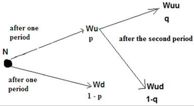
the second equated monthly installment at the above mentioned risk free interest rate.

Case II: ‘1-q’ is the probability of his default in the second period provided he did not default in the first period. In this case, the wealth of a bank would stand at ‘Wud’ at the end of the second period. Here, one may calculate ‘q’ by solving the equality Wu = q Wuu + (1-q) Wud.