A TYPICAL ONE-YEAR PROJECTION
The following one-year projection works through the effects of the analyst’s assumptions on all three basic financial statements. There is probably no better way than following the numbers in this manner to appreciate the
ăî
ăî
interrelatedness of the income statement, the cash flow statement, and the balance sheet.
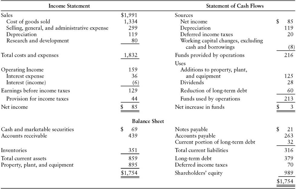
Exhibit 12.1 displays the current financial statements of a fictitious company, Colossal Chemical Corporation.
The historical statements constitute a starting point for the projection by affirming the reasonableness of assumptions about future financial performance. It will be assumed throughout the commentary on the Colossal Chemical projection that the analyst has studied the company’s results over not only the preceding year but also over the past several years.Projected Income Statement
The financial projection begins with an earnings forecast (Exhibit 12.2). Two key figures from the projected income statement, net income and depreciation, will later be incorporated into a projected statement of cash flows. The cash flow statement, in turn, will supply data for constructing a projected balance sheet. At each succeeding stage, the analyst will have to make additional assumptions. The logical flow, however, begins with a forecast of earnings, which will significantly shape the appearance of all three statements.
EXHIBIT 12.2 Earnings Forecast
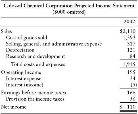
Immediately following is a discussion of the assumptions underlying each line in the income statement, presented in order from top (sales) to bottom (net income).
Sales The projected $2.110 billion for 2002 represents an assumed rise of 6% over the actual figure for 2001 shown in Exhibit 12.1.
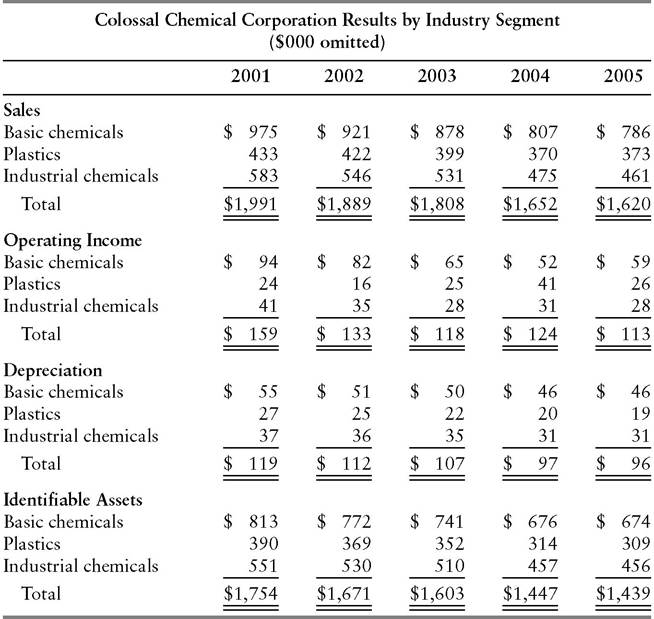
Of this increase, higher shipments will account for 2% and higher prices for 4%.To arrive at these figures, the analyst builds a forecast “from the ground up,” using the historical segment data shown in Exhibit 12.3. Sales projections for the company’s business, basic chemicals, plastics, and industrial chemicals, can be developed with the help of such sources as trade publications, trade associations, and firms that sell econometric forecasting models.
EXHIBIT 12.3 Sales Forecast
Certain assumptions about economic growth (increase in gross domestic product) in the coming year underlie all such forecasts. The analyst must be careful to ascertain the forecaster’s underlying assumptions and judge whether they seem realistic.
If the analyst is expected to produce an earnings projection that is consistent with an in-house economic forecast, then it will be critical to establish a historical relationship between key indicators and the shipments of the company’s various business segments. For example, a particular segment’s shipments may have historically grown at 1.5 times the rate of industrial production or have fluctuated in essentially direct proportion to housing starts. Similarly, price increases should be linked to the expected inflation level. Depending on the product, this will be represented by either the Consumer Price Index or the Producer Price Index.
Basic industries such as chemicals, paper, and capital goods tend to lend themselves best to the macroeconomic-based approach described here. In technology-driven industries and “hits-driven” businesses such as motion pictures and toys, the connection between sales and the general economic trend will tend to be looser.
Forecasting in such circumstances depends largely on developing contacts within the industry being studied. The objective is to make intelligent guesses about the probable success of a company’s new products.A history of sales by geographic area (Exhibit 12.4) provides another input into the sales projection. An analyst can modify the figures derived
EXHIBIT 12.4 Colossal Chemical Corporation Results by Geographic Area ($000 omitted)
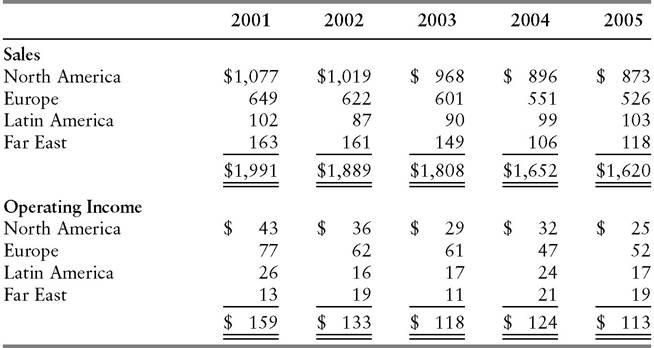
from industry segment forecasts to reflect expectations of unusually strong or unusually weak economic performance in a particular region of the globe. Likewise, a company may be experiencing an unusual problem in a certain region, such as a dispute with a foreign government. The geographic sales breakdown can furnish some insight into the magnitude of the expected impact of such occurrences.
Cost of Goods Sold The $1,393-billion cost-of-goods-sold figure in Exhibit 12.2 represents 66% of projected sales. That corresponds to a gross margin of 34%, a slight improvement over the preceding year’s 33%. The projected gross margin for a company in turn reflects expectations about changes in costs of labor and material. Also influencing the gross margin forecast is the expected intensity of industry competition, which affects a company’s ability to pass cost increases on to customers or to retain cost decreases.
In a capital-intensive business such as basic chemicals, the projected capacity utilization percentage (for both the company and the industry) is a key variable. At full capacity, fixed costs are spread out over the largest possible volume, so unit costs are minimized.
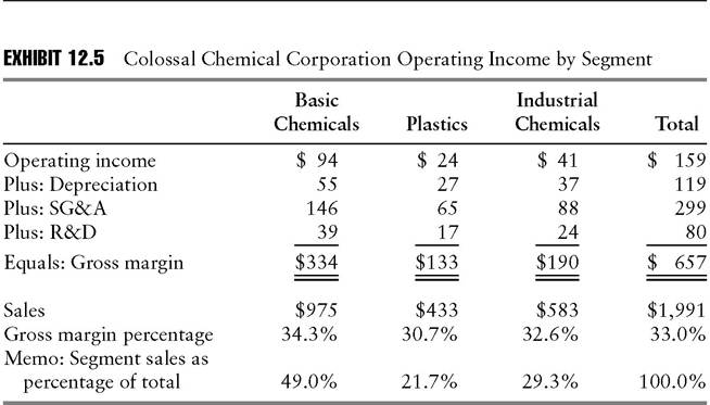
Furthermore, if demand exceeds capacity so that all producers are running flat out, none will have an incentive to increase volume by cutting prices. When such conditions prevail, cost increases will be fully (or more than fully) passed on and gross margins will widen. That will be the result, at least, until new industry capacity is built, bringing supply and demand back into balance. Conversely, if demand were expected to fall rather than rise in 2002, leading to a decline in capacity utilization, Exhibit 12.2’s projected gross margin would probably be lower than in 2001, rather than higher. (For further discussion of the interaction of fixed and variable costs, see Chapter 3.)As with sales, the analyst can project cost of goods sold from the bottom up, segment by segment. Since the segment information in Exhibit 12.3 shows only operating income, and not gross margin, the analyst must add segment depreciation to operating income, then make assumptions about the allocation of selling, general, and administrative expense and research and development expense by segment. For example, operating income by segment for 2001 works out as shown in Exhibit 12.5, if SG&A and R&D expenses are allocated in proportion to segment sales.
class=a7 style='text-indent:18.0pt'>By compiling the requisite data for a period of several years, the analyst can devise models for forecasting gross margin p ercentage on a segment-by- segment basis.Selling, General, and Administrative Expense The forecast in Exhibit 12.2 assumes continuation of a stable relationship in which SG&A expense has historically approximated 15% of sales. The analyst would vary this percentage
for forecasting purposes if, for example, recent quarterly income statements or comments by reliable industry sources indicated a trend to a higher or lower level.
Depreciation Depreciation expense is essentially a function of the amount of a company’s fixed assets and the average number of years over which it writes them off.
If on average, all classes of the company’s property, plant, and equipment (PP&E) are depreciated over eight years, then on a straightline basis the company will write off one-eighth (12.5%) each year. From year to year, the base of depreciable assets will grow to the extent that additions to PP&E exceed depreciation charges.Exhibit 12.2 forecasts depreciation expenses equivalent to 13.5% of PP&E as of the preceding year-end, based on a stable ratio between the two items over an extended period. Naturally, a projection should incorporate any foreseeable variances from historical patterns. For example, a company may lengthen or shorten its average write-off period, either because it becomes more liberal or more conservative in its accounting practices, or because such adjustments are warranted by changes in the rate of obsolescence of equipment. Also, a company’s mix of assets may change. The average write-off period should gradually decline as comparatively short-lived assets, such as data-processing equipment, increase as a percentage of capital expenditures and long-lived assets, such as “bricks and mortar,” decline.
Research and Development R&D, along with advertising, is an expense that is typically budgeted on a percentage-of-sales basis. The R&D percentage may change if, for example, the company makes a sizable acquisition in an
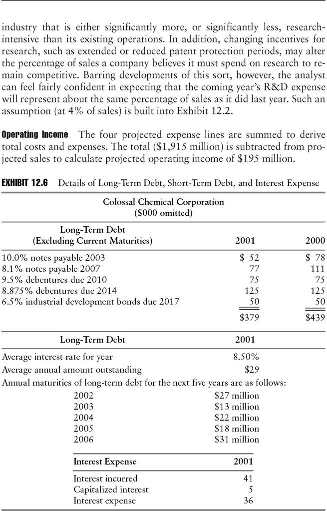
Interest Expense Exhibit 12.6 displays information found in the Notes to Financial Statements that can be used to estimate the coming year’s interest expense. (Not every annual report provides the amount of detail shown here. Greater reliance on assumptions is required when the information is sketchier.)
The key to the forecasting method employed here is to estimate Colossal Chemical’s embedded cost of debt, that is, the weighted average interest rate on the company’s existing long-term debt.
Using the details of individual long-term issues shown in Exhibit 12.5, the calculation goes as follows: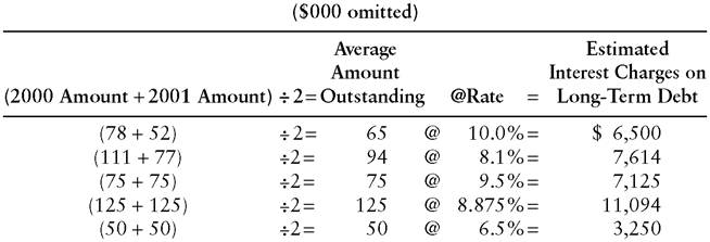
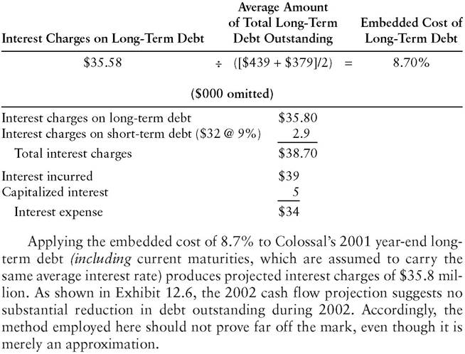
To the $35.8-million figure, the forecaster must add interest charges related to the short-term debt. These projections assume an average outstanding balance of $32 million, 10% higher than in 2001. The assumed average interest rate is 9%, based on an expectation of slightly higher rates in 2002:

The $38.7-million figure represents total interest that Colossal is expected to incur in 2002. From this amount, the forecaster must subtract an assumed level of capitalized interest to obtain projected interest expense. Exhibit 12.2 simply projects capitalized interest at the same level in 2002 as in 2001:
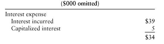
Readers should bear in mind that the method described here for projecting interest expense involves a certain amount of simplification. Applied retroactively, it will not necessarily produce the precise interest expense shown in the historical financial statements. For one thing, paydowns of long-term debt will not come uniformly at midyear, as implicitly assumed by the estimation procedure for average amounts of long-term debt outstanding. Certainly, analysts should recognize and adjust for major, foreseeable changes in interest costs, such as refinancing of high-coupon bonds with cheaper borrowings. By the same token, forecasters should not go overboard in seeking precision on this particular item. For conservatively capitalized industrial corporations, interest expense typically runs in the range of 1% to 2% of sales, so a 10% error in estimating the item will have little impact on the net earnings forecast. Analysts should reserve their energy in projecting interest expense for more highly leveraged companies. Their financial viability may depend on the size of the interest expense “nut” they must cover each quarter.
class=a7 style='text-indent:0cm'>Interest Income Exhibit 12.2 incorporates a forecast of an unchanged cash balance for 1995. Based on expectations of an average money market rate of return of 7.0% on corporate cash, the average balance of $69 million will generate (in round figures) $5 million of interest income.Provision for Income Taxes Following the deduction of interest expense and the addition of interest income, earnings before income taxes stand at $166 million. The forecast reduces this figure by the statutory tax rate of 34%, based on Colossal’s effective rate having historically approximated the statutory rate. For other companies, effective rates could vary widely as a result of tax loss carryforwards and investment tax credits, among other items. Management will ordinarily be able to provide some guidance regarding major changes in the effective rate, while changes in the statutory rate are widely publicized by media coverage of federal tax legislation.
Projected Statement of Cash Flows
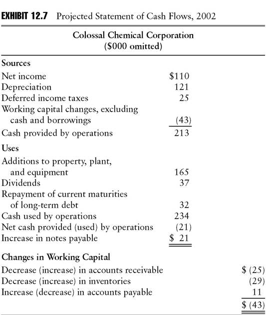
The completed income statement projection supplies the first two lines of the projected statement of cash flows (Exhibit 12.7). Net income of $110 million and depreciation of $121 million come directly from Exhibit 12.2 and largely determine the total sources (funds provided by operations) figure. The other two items have only a small impact on the projections.
Deferred Income Taxes This figure can vary somewhat unpredictably from year to year, based on changes in the gap between tax and book depreciation and miscellaneous factors such as leases, installment receivables, and unremitted earnings of foreign subsidiaries. Input from company management may help in the forecasting of this figure. The $25-million figure shown in Exhibit 12.7 is a trend-line projection.
Working Capital Changes (Excluding Cash and Borrowings) Details of the derivation of the $43-million projection appear at the bottom of Exhibit 12.7. The forecast assumes that each working capital item remains at the same percentage of sales shown in the historical statements in Exhibit 12.1. Accounts receivable, for example, at 22% of sales, rises from $439 million to $464 million (an increase of $25 million) as sales grow from $1,991 million in 2001 to a projected $2,110 million in 2002. Before assuming a constantpercentage relationship, the analyst must verify that the most recent year’s ratios are representative of experience over several years. Potential future deviations from historical norms must likewise be considered. For example, a sharp drop in sales may produce involuntary inventory accumulation or a
rise in accounts receivable as the company attempts to stimulate its sales by offering easier credit terms.
Additions to Property, Plant, and Equipment The first and largest of the uses on this cash flow projection is capital expenditures. A company may provide a specific capital spending projection in its annual report, then, as the year progresses, update its estimate in its quarterly statements or 10-Q reports and in press releases. Even if the company does not publish a specific number, its investor-relations officer will ordinarily respond to questions about the range, or at least the direction (up, down, or flat) for the coming year.
Dividends The $37-million figure shown assumes that Colossal will continue its stated policy of paying out in dividends approximately one-third of its sustainable earnings (excluding extraordinary gains and losses). Typically, this sort of guideline is interpreted as an average payout over time, so that the dividend rate does not fluctuate over a normal business cycle to the same extent that earnings do. A company may even avoid cutting its dividend through a year or more of losses, borrowing to maintain the payout if necessary. This practice often invites criticism and may stir debate within the board of directors, where the authority to declare dividends resides.
Until the board officially announces its decision, an analyst attempting to project future dividends can make only an educated guess. In a difficult earnings environment, moreover, a decision to maintain the dividend in one quarter is no assurance that the board will decide the same way three months later.
Repayment of Current Maturities of Long-Term Debt The $32-million figure shown comes directly from the current liabilities section of the balance sheet in Exhibit 12.1.
Increase in Notes Payable Subtracting $234 million of cash used in operations from the $213 million provided by operations produces a net use of $21 million. This projection assumes that any net cash generated will be applied to debt retirement. A net cash use, on the other hand, will be made up through drawing down short-term bank lines. Underlying these assumptions about the company’s actions are management’s stated objectives and some knowledge of how faithfully management has stuck to its plans in the past. Other assumptions might be more appropriate in other circumstances. For example, a net provision or use of cash might be offset by a reduction or increase in cash and marketable securities. A sizable net cash provision might be presumed to be directed toward share repurchase, reducing shareholders’ equity, if management has indicated a desire to buy in stock and is authorized to do so by its board of directors. Instead of making up a large cash shortfall with short-term debt, a company might instead fund the borrowings as quickly as possible (add to its long-term debt). Alternatively, a company may have a practice of financing any large cash need with a combination of long-term debt and equity, using the proportions of each that are required to keep its ratio of debt to equity at some constant level.
Projected Balance Sheet
Constructing the projected balance sheet (Exhibit 12.8) requires no additional assumptions beyond those made in projecting the income statement and statement of cash flows. The analyst simply updates the historical balance sheet in Exhibit 12.1 on the basis of information drawn from the other statements.
EXHIBIT 12.8 Colossal Chemical Corporation Projected Balance Sheet December 31, 2002 ($000 omitted)
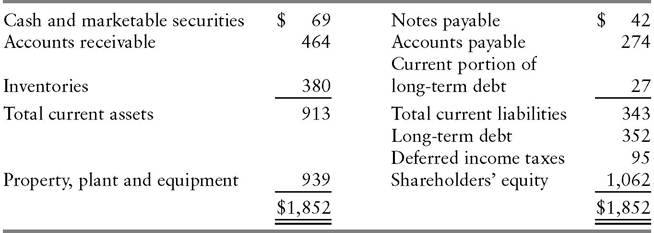
Most of the required information appears in the projected statement of cash flows (Exhibit 12.7). Accounts receivable, inventories, and accounts payable, for example, reflect the projected changes in working capital. The cash flow projection would likewise show any increase or decrease in cash and marketable securities, an item that in this case remains flat. Property, plant, and equipment rises from the prior year’s level of $895 million by $165 million of additions, less $121 million of depreciation. The projected cash flow statement also furnishes the increases in notes payable and deferred income taxes, as well as the change in shareholders’ equity (net income less dividends).
The details of long-term debt in the historical balance sheet (Exhibit 12.6) provide the figures needed to complete the projection of long-term debt. With the 2001 current maturities of long-term debt ($32 million) having been paid off, the 2002 current maturities ($27 million) take their place on the balance sheet. The $27-million figure is also deducted from 2001’s (noncurrent) long-term debt of $379 million to produce the new figure of $352 million. (Any further adjustments to long-term debt, of which there are none in these projections, would appear in the projected statement of cash flows.)