Competition in other 2-consumer-l-resource models
While the MacArthur consumer-resource model with all-linear component functions is very widely used, at least two other types of components have frequently
Competition in seasonal environments: temporal overlap • 201 been employed in competition theory; (1) models with abiotic (chemostat) resource dynamics; and (2) models in which the consumer functional response is type II.
The former has fewer possibilities for large delays in the resource dynamics, while the latter has more such possibilities, as well as the possibility of self-sustaining cycles in the absence of seasonality. When either of these alternative scenarios is adopted in seasonal models, the dynamics change significantly. The combination of biotic resources and type II responses creates an interaction of the exogenous and endogenous periodicities, which is known to produce complex dynamics in1- consumer-1-resource systems (Rinaldi et al. 1993, Sauve et al. 2020). In the
2- consumer-2-resource case, both of these alternative assumptions also produce a wide range of dynamical behaviours, including cases having alternative exclusion as the only outcome, and other cases with both exclusion and coexistence outcomes. Exclusion due to temporal partitioning is again associated with consumer dynamics that are not much slower than the resource dynamics and a relatively short seasonal period (equivalently, slow dynamics of all species). Here I will again just provide a few examples that illustrate some of the similarities and differences of these alternative models from the ones examined earlier in the chapter. All of these models deserve a much more comprehensive analysis.
8.3.1 Systems with abiotic resources
The dynamics of competitive systems having abiotic resources are usually simpler than those with biotic resources, and differences in seasonal responses are more likely to promote coexistence.
However, there is still a lag in the response of the resource abundance to temporal cycles in consumption, and this can still lead to a failure of seasonal partitioning to produce coexistence, as well as producing various dynamic complexities. Relatively high resource exit rate parameters imply strong stabilization, so the following examples have low values of E in the abiotic growth function, I - ER. Table 8.6 describes the dynamical outcomes for an example that displays a wide range of outcomes as the period length q is increased. The qualitative outcomes here have many similarities with the logistic resource results presented in Section 8.2. A broad range of relatively low period lengths produce only alternative exclusion, and sufficiently long periods produce coexistence with anti-synchronized cycles. Intermediate periods can produce two alternative coexistence equilibria in which one species has a greater average abundance than the other, or a single coexistence attractor with aperiodic variation.If the Table 8.6 system is changed to have a smaller death rate (equal for both consumers), the upper boundary of the range of q producing alternative exclusion is reduced; i.e., coexistence is favoured. The opposite is true for death rates greater than that in Table 8.6). As in the model with logistic resources, there are abrupt changes in the limiting dynamics with changes in the mortality rate of one consumer species. Even without abrupt changes, measures of interspecific effects change greatly
Table 8.6 Outcomes in the abiotic resource-linear functional response model {parameters:
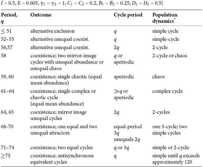
* Cycles are classified by number of maxima in abundance for the more abundant (or both) consumer species during the course of the cycle (where ‘simple' denotes 1 peak per species per period q). Equal and unequal refer to the mean consumer abundances.
as the mortality rate of one species is increased from the minimum to the maximum allowing coexistence.
Cases similar to that considered in Table 8.6 are also characterized by similar possibilities for exclusion or coexistence when an aseasonal species competes with a seasonal one that is otherwise equivalent. The seasonal species can prevent invasion by the aseasonal species or vice versa in the abiotic resource model provided that q < 52; for lower q, a seasonal consumer produces a lower mean resource density than the equilibrium resource density for the aseasonal one. However, for q ≥ 52, the aseasonal species always excludes the seasonal. This outcome for long environmental periods is sensitive to the exact equality of all of the mean fixed parameter values; if the aseasonal species has a slight disadvantage in one of the mean parameters (resulting in a higher mean resource abundance in a single-consumer system), it can coexist with the seasonal species in environments with long environmental periods (or equivalently, with rapid consumer and resource dynamical rates).
8.3.2 Biotic resources with type II functional responses
Another simple model assumes logistic resource growth and consumers that have type II (disc equation) functional responses. Here the resource capture rate of a consumer individual is given by CR∕(1 + ChR), where h is handling time. This adds the possibility of sustained cycles in the absence of seasonality. Seasonal systems with a single type II consumer species and a living resource are known to have a wide range of complicated dynamical behaviours due to interactions of the seasonal forcing and the forcing due to the inherent predator-prey cycle (King and Schaffer 1999; Sauve et al. 2020). This suggests that the range of dynamical patterns that can be observed in the 2-consumer case is likely greater than for either of the linear functional response models considered thus far in this chapter. However, the possibility of sustained or very slowly damped cycles in non-seasonal logistic-type II systems raises the possibility that these systems could display different responses to seasonal variation.
Sustained cycles in an aseasonal single-consumer system occur when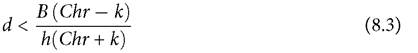
Thus, sustained cycles do not occur for any mortality rate when Chr/k < 1. For example if C = 1, this implies that an aseasonal system is stable for all d when h < k/r; i.e., h ≤ 0.005 when the other parameters are as in the Figure 8.3 example.
A type II response alters the nature of cycles in seasonal 1-consumer systems, even if sustained cycles do not occur in the aseasonal case having the same parameters. However, the broad pattern of coexistence and exclusion in a system of two antisynchronized competitors described above is often similar, at least for systems that have mortality rates slightly greater than the stability threshold given by eq. (8.3). If the Figure 8.3 example of a MacArthur model is changed to have h = 0.005 for each consumer, relatively short periods, q, usually produce alternative exclusion outcomes, and relatively long periods produce coexistence. The dividing line between these two outcomes occurs between periods of 67 and 68. The dynamics of this system are more often aperiodic than for the linear functional response system, and there are more frequent changes in the qualitative pattern of the dynamics with increasing q. The presence of a significant but low-level consumer immigration allows coexistence for a range of intermediate period lengths (roughly q between 22 and 28), and allows a range of alternative coexistence or exclusion outcomes for periods between 50 and 60. However, periods > 60 only produce coexistence. Doubling h to 0.01 in this example (with no consumer immigration) produces cyclic dynamics even in the absence of seasonal variation. However, the general impact of seasonal cycles on coexistence is similar to the previous case of h = 0,005; alternative exclusion for shorter periods, and coexistence for longer periods, with the switch occurring between q = 77 and q = 78.
8.3.2 Abiotic resources with type II functional responses
Here, the type II functional response does not destabilize the equilibrium in the absence of seasonal variation. The general pattern of alternative exclusion for low environmental periods and coexistence for greater periods continues to hold in this case for a system broadly similar to the previously considered linear functional response-abiotic resource model. It has parameters: I = 0.5, E = 0.005, γ1 = γ2 = 0.9; Ci = C2 = 0.2, h1 = h2 = 0.05; Bi = B2 = 0.05; D1 = D2 = 0.2, with L = q/2. Alternative exclusion outcomes occur from period lengths of q = 2 through q = 180; periods of 190 through 248 yield two ‘mirror image' attractors having unequal mean abundances for the two consumers. Periods of 250 and above yield coexistence with anti-synchronized cycles and equal mean consumer abundances.
8.4