A modelling framework and a seasonal MacArthur system
This section presents numerical analyses of examples of commonly used consumerresource models. The selection of specific examples is designed to illustrate the operation of general mechanisms using models that are familiar in a non-seasonal context.
8.2.1 General features of the models
The basic model has a single resource with abundance R, and a number of consumer species with abundance Ni for species i. It is:
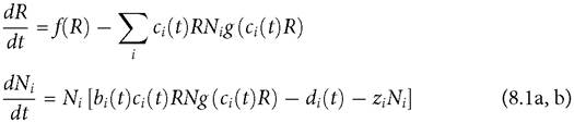
The function g represents effects of resource abundance on the baseline attack rate ci; the most common of these is the effect of handling time or satiation. If the consumers have linear functional responses g = 1; g = 1/(1 + c(t)hR) when the response is described by Hollings formula for a type II response, where h is the handling time required for each resource item. The function g is assumed to be identical across species to rule out differences in the linearity of the consumers’ responses as a factor generating coexistence. The three consumer parameters (b, c, d) are respectively resource conversion efficiency, resource attack rate (maximal per capita consumption rate), and per capita mortality rate. The analysis will examine seasonal variation in each of these three parameters. The parameter zi represents a per capita negative effect of species i on its own per capita growth rate. Such intraspecific interference terms can allow coexistence even in the absence of seasonality. In most of the analysis these zi parameters are assumed to equal zero. However, interference terms can be used to measure the strength of exclusion in cases where it occurs in the absence of interference. The function f is the resource growth rate. In the MacArthur model, f is the logistic growth function, g = 1, and z = 0.
The variation in parameters is modelled by multiplying the mean parameter (here denoted by capitals: Bi, Ci, or Di) by the following function:
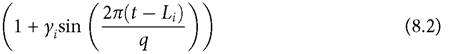
The parameter q is the period of the cycle, and Li is the lag in the variation experienced by species i relative to that experienced by species 1 (L1 = 0 and Li < q, by definition). The parameter γ (with 0 ≤ γ ≤ 1) adjusts the magnitude of the sinusoidal variation, from non-existent (γ = 0) to a value (γ = 1) large enough reduce the parameter to zero at the low point of the cycle. This framework implies a maximum parameter value of twice the mean. An extension of this model considered briefly below has two resources with equivalent growth parameters but different vulnerabilities to the consumer; this reveals the interaction of (structural) resource partitioning with seasonal partitioning. In the 2-resource analysis below, expression (8.2) multiplies each of the two mean capture rate parameters for species i, Ci1 and Ci 2.
For many, if not most, species the annual cycle of change in climatic variables causes changes in population growth parameters. Thus, some previous work (Li and Chesson 2016) has measured time in years and has been limited to the case of q = 1. However, there are multi-year cycles and quasi-cycles in climatic variable (e.g. the Pacific decadal oscillation). Even for annual cycles, q obviously takes on values greater than one if the timescale used to measure the other rate constants in the model is less than annual. The fundamental issue is the relative speeds of the population dynamics (of all species) and seasonal change. Greater change in population abundances within a season can be produced by either longer seasons or more rapid population dynamics (of both species). An increase in q is equivalent to maintaining q = 1 and increasing the set of rate constants, r, k, C, and d, by the same factor; q is thus simply a scaling factor for the four temporal rate constants.
In Hutchinson’s (1961) famous example of plankton, an annual cycle often involves several reversals in the relative abundances of all of the species concerned due to their rapid dynamics (see Figure 1 of Sommer et al. 2012). This implies q >> 1.1 concentrate on anti-synchronized cycles; L = q/2. This minimizes the temporal parameter overlap of two species with sinusoidal variation in resource-related parameters.The most commonly used functions for resource growth are the logistic and the linear abiotic (‘chemostat’) models. The versions of these models used here are respectively given by f (R) = m +R(r - kR), and f (R) = I - ER. In the logistic model r is the maximum per capita rate of increase, and k is the per capita density-dependent reduction in that rate; m is an input due to external immigration, and a (small) positive value of m is appropriate when the system is part of a larger metacommunity. In the abiotic model, I is the rate of input, and E is the per capita loss rate. (Any external input from other patches can be included in I.) Because of its prominence in previous theory, I will concentrate on the ‘MacArthur’ system (MacArthur 1970, 1972; Chesson 1990, 2020a, b), which assumes a logistic resource and a linear consumer functional response. Some models with two resources will be considered to compare the impacts of temporal partitioning due to seasonality to the impacts of strict resource-type partitioning. These simple models are inadequate representations of almost any natural system (Abrams 1988a, 2010b), but there is no reason to believe they produce an unusually wide range of sensitivities to seasonal forcing.
Understanding the impact of environmental variation is complicated because of the interaction of the periodicity of the environment with the inherent periodicity of the consumer-resource interaction. These interacting periodicities produce the complicated range of dynamics found in seasonal predator-prey models (Rinaldi et al. 1993; King and Schaffer 1999; Sauve et al.
2020). As shown in the following section (8.2.2), it is possible for the environmental fluctuations to produce a positive effect on a single resident consumer when the recovery of the resource (prey) from heavy consumption coincides with the consumer’s (predator’s) period of greatest consumption or conversion rate. Such situations are reflected in a lower mean resource abundance than in a constant environment. The analysis begins with an examination of lags and resource dynamics in a system having only a single consumer (and a single logistic resource).8.2.2 Resource lags and mutual Invasibility of MacArthur systems
The response of both resource and consumer populations to an instantaneous change in a consumer rate parameter takes a finite amount of time to be fully realized. The duration of these lags and the pattern of seasonal variation jointly determine the resource abundance at any given time in the future. A rough indication of the effect of lagged resource changes on consumer dynamics can be seen in Figure 8.1, which plots the resource abundance and the consumer’s scaled per capita capture rate (c(t)) in eqs (8.1) as a function of time in a periodic environment for the MacArthur consumer-resource model, with both species exhibiting their limiting dynamics. Resource abundance is shown in blue, resident consumer c(t) is dashed-black.
The plot also shows the c(t) curve of a rare competitor (dashed-red) whose response to the environment is 180 degrees behind that of the first species. (The c-curves have been multiplied by 10 for visual comparison with the much larger resource density.)
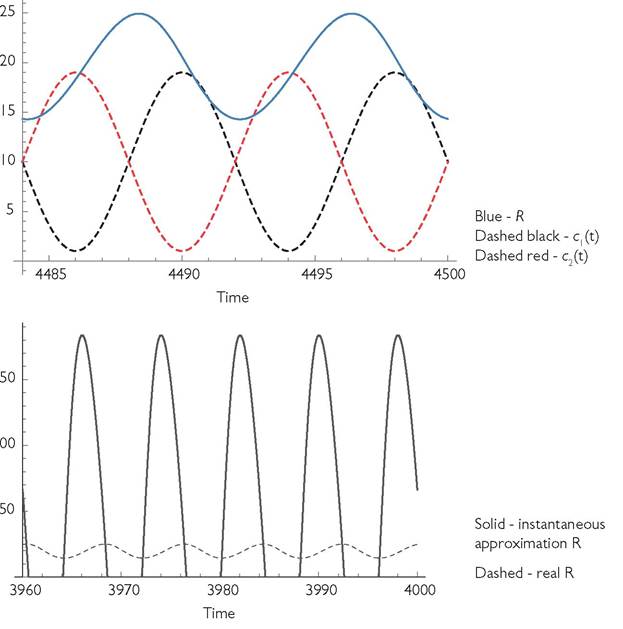
Fig. 8.1 Panel A. Resource dynamics (solid blue) and the dynamics of the intake rate parameters c(t) for two anti-synchronized consumer species in the MacArthur model; the resident consumer’s c(t) is given by the black dashed line, and the invader by the red dashed line; both have been multiplied by a factor of 10 to make them easily visible on the scale of the graph.
The parameters are: r = 0.25; k = 0.00125; γ1 = γ2 = 0.9; C1 = C2 = 1; b1 = b2= 0.01; d1 = d2 = 0.2; m = 0.001; q = 8, L = 4.Panel B. This gives the resource curve from panel A (dashed) together with the hypothetical resource curve that would apply if the resource achieved equilibrium instantaneously with respect to the actual consumer abundance at all times in the system from panel A (negative values are omitted). The (hypothetical) negative resource abundances occur because the consumer abundance reaches higher levels than it would if the resource actually did achieve equilibrium instantaneously. This shows the inadequacy of the assumption of immediate resource equilibration in this system.
The resident’s c(t) curve is more closely correlated with resource abundance than is the invader’s c(t); this can be seen by comparing the resource abundance at the peaks of the two c(t) curves. The resulting lower resource intake of the invader implies a negative mean per capita growth rate, since the resident’s mean is zero at its limiting dynamics. Thus the invader is excluded. The roles of resident and invader are arbitrary here, meaning that either species can exclude the other. Figure 8.1B shows the resource abundances that would occur if the resource abundance were to immediately reach its equilibrium for the actual consumer abundances in this system; this is presented to show how misleading such an assumption would be here.
The per capita rate of increase of an invader with a different lag (but otherwise equivalent parameters) can easily be calculated from the resource abundance curve shown in Figure 8.1A. That invasion curve is shown in Figure 8.2A. This figure shows that the invader (say species 2) must have a lag of slightly greater than 4.5 to increase when rare; this is greater than 1/2 the period length (q = 8). Because the invader and resident roles are interchangeable with a q/2 phase shift under this scenario, if invasion of one competitor is impossible for all lags < q/2, symmetry implies that mutual invasion of two otherwise equivalent species is impossible for any lag.
If invasion density is low enough, the starting point of the environmental cycle will not significantly affect invasion success. In Figure 8.2, an invader that has a lag somewhat greater than 1/4 period (L = 2.2767 in Figure 8.1) has the lowest fitness of any invading type. The invasion curve implies that invasion of a ‘later’ consumer becomes more difficult as lags increase from 0 to 2.2767; a still larger L increases invasion fitness, which becomes positive at a lag of 4.552. Figure 8.2A shows that, if species 2 had a mortality rate that was lower than that of species 1 by 0.02, it could invade if its lag were less than approximately 1.20, but not for any lags between 1.20 and 3.42. In other words, it is possible for greater differences in seasonal timing to make invasion impossible when shorter lags make it possible. The reverse is possible as well. In general, the failure of mutual invasion need not rule out coexistence, although it is impossible in the system illustrated in Figure 8.2. No coexistence attractor was observed for any integer q < 20 in this system.Coexistence with mutual invasibility is possible for a range of lags when resource dynamics are more rapid relative to consumer dynamics. If the resource parameters r and k are each multiplied by 10 in the Figure 8.2A example, the invasion curve becomes that shown in Figure 8.2B. This figure implies that lags between approximately 1.5 and 6.5 allow mutual invasibility. Plots like those in Figures 8.2A, B differ in form depending on the length of the environmental period, and the demographic parameters of both species. If the dynamics of both species are sufficiently rapid (equivalently, if the period q is sufficiently long) then species with anti-synchronized seasonal cycles in their attack rates will always coexist in this model. However, for a broad range of short to moderate period lengths (with other parameters as in Figures 8.2A, B), coexistence of any pair of seasonally offset but otherwise equivalent competitors is not possible.
Temporal correlation between relatively high resource abundance and relatively high consumer capture rate in a seasonally varying consumer species produces an
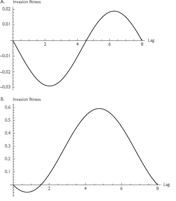
Fig. 8.2 Panel A. 'The per capita growth rate of a very rare (lagged) invader in the MacArthur system (eqs (8.1)) with the parameters (other than L) given in Figure 8.1, having a resident species undergoing its limiting population cycle. The invasion rate is given for invaders characterized by different lags, L.
Panel B. As in panel A, except that r and k have been multiplied by 10. The invasion rate is given for invaders characterized by different lags, L.
average resource abundance that is lower than the equilibrium value for an equivalent aseasonal consumer, preventing its invasion. It also prevents invasion for a range of seasonal consumer types that differ from the resident only in the lag of their seasonal c(t) curves, including an anti-synchronized species. However, it is always possible for an otherwise identical consumer with a slightly earlier c(t) curve (L slightly less than q) to invade and displace the resident, unless it suffers some lowered mean parameter as a consequence of that earlier timing. If the timing of the original resident is adaptive this implies that early individuals will have lower mean values of one or more fitness parameters, and this may be large enough to outweigh the advantage of earlier resource exploitation. Lags that are small enough relative to q always result in exclusion of the lagged invader unless it has some advantage in mean fitness parameters.
The ability of an anti-synchronized invader to increase when rare in the MacArthur model can be determined from the mean resource abundance in the resident-only system, once it has reached its limiting dynamics. Mean resource abundance less than the equilibrium for an otherwise equivalent aseasonal species implies that the aseasonal invader would be unable to increase when rare. As noted above, the mean resource abundance is also an accurate indicator of the outcome of competition with an anti-synchronized competitor, which will be discussed first. This equivalence is due to the fact that the per capita growth rate function is linear, and the seasonal term is equal and opposite at all points in time for the resident and antisynchronized invader. For the resident undergoing its limiting dynamics, the mean per capita growth rate must be zero. Thus, meanR] = d/BC mean[γsin[2πt /q])R]. If the mean R in the resident-only system is less than its aseasonal equilibrium of d/BC, this implies that mean[γsin[2πt /q])R] > 0. The anti-synchronized invader's per capita growth is BC(1 + γsin[2π(t--(q/2))/q ])R ]--d. Because the value of the antisynchronized sine function is the negative of its original value, the invasion condition becomes BC(1-γsin[2πt7q])R-d > 0. This cannot be satisfied if mean[R] is less than its aseasonal equilibrium of d/(BC). Note that the amplitude of the change in c(t), given by γ, does not alter the condition for invasion from low density for an otherwise equivalent anti-synchronized competitor, although it does modify the magnitude of the invasion growth rate.
Whether the mean resource density is greater or less than the aseasonal equilibrium value is determined by the seasonal period, q. (Recall that a larger q is equivalent to proportional increases in all rate parameters of the two species; r, k, c, and d.) The mean R, in turn, determines whether there are mutual exclusion outcomes for two anti-synchronized competitors. Figure 8.3 shows the mean R for a range of period lengths (q) in a single-consumer system that is otherwise identical to the one assumed in Figures 8.1 and 8.2A. The range of periods shown encompasses the range of qualitatively different dynamics produced. The period lengths associated with two or more dots at a given q have alternative attractors, characterized by different mean R. The alternative attractors for each period were found by continuing all known attractors occurring at higher or lower q and by starting each parameter set from five randomly chosen starting abundances from the interval between 0 and twice the aseasonal equilibrium population size for each species. This numerical search method does not ensure that all possible attractors have been located, but it has a good chance of locating most of those with significant basins of attraction. The population dynamics observed for the lowest range of period lengths (q < 10) consists of a simple cycle with period q. The majority of the longer periods illustrated, starting with q = 11, have at least two alternative population cycles.
The environmental period lengths, q, associated with alternative attractors often have an attractor with period q and another which is a small integer multiple of q.
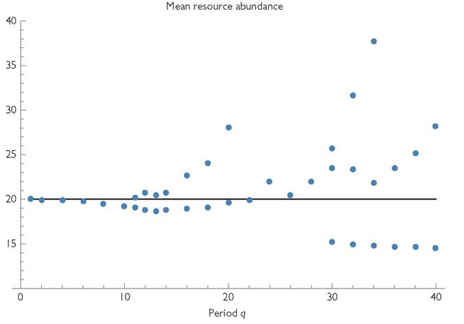
Fig. 8.3 'The mean resource abundance (blue dots) in a consumer-resource (predatorprey) system for a range of seasonal periods, q. This system is otherwise identical to that in Figures 8.1 and 8.2. (Parameters are: r = 0.25; k = 0.00125; γ1 = 0.9; C1 = 1; b1 = 0.01; d1 = 0.2; m = 0.001) The black line gives the equilibrium resource abundance for the same system in the absence of any variation. Note that only integer periods were studied, and only even integers were simulated for most of the range shown.
Aperiodic population variation also occurs for some values of q. The seasonal period lengths with a mean resource density much lower than the aseasonal equilibrium of R = 20 that characterizes q between 30 and 40 are all simple cycles with period q. The attractors having longer period population cycles within this range of q have mean resource densities > 20; this implies that they can be invaded by an antisynchronized competitor. Because of the irregular forms of the dynamics that occur for q = 18 through 23, determining an accurate mean abundance may require averaging over an extremely long temporal interval, and for some significant part of this interval, the mean resource abundance may be significantly greater or less than the long-term mean. This has the potential to make invasion success dependent upon initial abundance of the invader.
Periods moderately longer than the largest q (= 40) shown in Figure 8.3 are mostly characterized by population cycles with the environmental period, q. For sufficiently long periods, there are two or more local population maxima per cycle in each consumer species. An environmental period of 60 is the smallest integer period > 40 that lacks any attractor with a resource density less than the equilibrium of 20. All q >60 have mean resource densities > 20, implying coexistence with an anti-synchronized competitor. Integer values of q of 69 through 76 have two or three alternative attractors with one, two, or four local maxima in abundance per period. Periods of 77 and 78 appear to be the largest environmental periods having population cycles that are longer than q (2q in this case). Environmental periods of 79 and greater imply at least two local maxima in consumer population size per period.
8.2.3 Coexistence in a 2-consumer MacArthur system
The dynamics of single-consumer systems described in Section 8.2.2 suggest that alternative exclusion occurs at sufficiently short periods (equivalently, slow dynamics of both species), and coexistence for sufficiently long periods. Outcomes for intermediate period lengths are more complicated, and require numerical exploration. The outcomes of simulations for a range of q in the anti-synchronized Figure 8.3 example are shown in Table 8.1. Figure 8.4 illustrates a small number of these cases. The most common qualitative outcomes are: (1) alternative exclusion only, for small q; (2) coexistence with irregular dynamics for low intermediate q; (3) alternative exclusion or coexistence with equal mean densities for high intermediate q; and (4) coexistence with equal mean densities for sufficiently large q. The dynamics within each category can exhibit a wide range of forms and cycle lengths and can be aperiodic. There are a number of values of q that do not fit this rough categorization; a range of period lengths (30 through 34) between categories (2) and (3) only exhibit alternative exclusion. As noted above, when the 1-consumer system has a single attractor for a given environmental period, the ability of an anti-synchronized competitor to invade from low density is determined by whether the resident produces a mean resource above or below the aseasonal equilibrium (20 in this case). Note that the initial population size and time of arrival for the invading species can be important in the outcome (given two or more attractors), since an initially much less abundant species may become more abundant during the first part of the post-invasion period if conditions at t = 0 give it a sufficient advantage over its competitor.
There is often a single outcome of these 2-consumer competition models for cases in which the corresponding single-species model has alternative outcomes. For periods of q = 11 through 18, there are two attractors for the initial resident consumer species, having mean resource abundances on either side of the equilibrium value of 20. If the resident occupies an attractor with mean resource abundance > 20, the invader initially increases. However, numerical integration shows that the growth of the invader shifts the dynamics of the resident to its other attractor, which then causes extinction of the invader. This makes it impossible for the initial invader to re-invade. For example, when q = 12 in a single-consumer system, there is an attractor with a period 12 cycle in abundances characterized by mean R < 20, and a second attractor with a higher-amplitude period 36 population cycle characterized by a mean R of 20.73. The initial increase of an anti-synchronized rare invader into this second resident attractor eventually shifts the resident dynamics as shown in Figure 8.5
(roughly around t = 200). This results in the exclusion of the invader. The outcome is similar for all periods 11 ≤ q ≤ 18, which have two attractors with mean resource abundances above and below R = 20. Thus, all systems having integer periods q by pronounced numerical dominance by one species were shortened and the minimum densities (which were many orders of magnitude less than the equilibrium) were increased by low- level immigration. This immigration also has a significant effect on the dynamics of
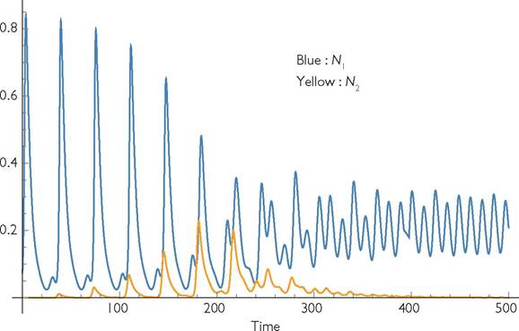
Fig. 8.5 The time course of consumer densities in a system where consumer species 1 (Nι, blue) has the parameters given under Figure 8.3. The seasonal period is q = 12. Consumer 2 has growth parameters identical to species 1 (γ2 = 0.9; C2 = 1; b2 = 0.01; d2 = 0.2), except it is anti-synchronous; i.e., L = 6 for species 2. The plot shows the outcome when a small number of consumer 2 is introduced into a system where consumer 1 is undergoing the period-36 cycles represented by the higher dot above q = 12 in Figure 8.3.
systems that are close to, but outside of, the range of periods allowing coexistence in the absence of consumer immigration. For example, if q = 19, immigration at a rate of 0.00001 for both consumers allows the initially less common species to persist at an average abundance approximately 1/16 that of the dominant species, rather than being excluded. Holt et al. (2003) discussed similar cases, in which a low level of immigration of a species into a ‘sink’ habitat can maintain significant abundances.
Larger rates of consumer immigration can eliminate the possibility of (quasi-) exclusion outcomes for some periods in the interval from 36 to 58, which has alternative exclusion and coexistence outcomes in the absence of consumer immigration. In this range of periods, greater immigration and longer periods both act to eliminate the exclusion outcomes. For example, q = 40 produces coexistence from all initial conditions when the consumer immigration rate is 0.001. However, when the immigration rate is 0.0001, coexistence and exclusion are both possibilities. Even when immigration is 0.0001, exclusion does not occur for q ≥ 52.
This complicated catalogue of dynamic outcomes has many features that are incompatible with techniques of ‘modern competition theory’, such as invasion analysis. They also show that temporal resource segregation has many possible relationships to coexistence having no analogue in traditional partitioning in temporally constant environments.
8.2.4 How robust and representative is the example?
The above results are a ‘best case scenario' for coexistence, in that consumers have equal parameters and anti-synchronized seasonality. The robustness of the exclusion outcomes may be explored by adding direct consumer interference (z > 0 in eq. (8.1)). When each of two or more consumers has purely intraspecific interference, this favours coexistence, and the magnitude of the interference, z, required for coexistence provides an index of the robustness of the exclusion outcomes. In the system considered in Figure 8.3, if q = 30, the maximum z that permits exclusion is 0.2251; at this point interference represents an increase of approximately 16% to the per capita death rate. Short environmental periods (or rapid dynamics of both species) produce small effects on the mean resource abundance, and these can be overcome by relatively small intraspecific interference effects. For example, a period of q = 6 always produces coexistence if z > 0.0135, Whichrepresents only a 3% increase in the mortality rate.
All of the above is based on a single set of parameters for the underlying aseasonal model. Li and Chesson (2016) have used the same MacArthur system with sinusoidal seasonal variation in c to illustrate how such variation promotes coexistence. An obvious question is whether the negative effects on coexistence shown here are restricted to a narrow range of the other parameters. Because a large enough q always produces coexistence, I examined this question for q = 10, as this is in the middle of the range of relatively low environmental periods that only exhibited alternative exclusion. I will describe how coexistence is affected by changing the consumer parameters (B, C, d) from the values they have in the example above. Each of these parameters may be increased or decreased by a large amount without changing the qualitative form of the outcome. Values of d from 0.02 to 1.8 were examined (the original system assumed d = 0.2). All d values within this range only produced alternative exclusion outcomes. Values of B between 0.00125 and 0.1 were simulated (baseline B = 0.01); only large B values between roughly 0.08 and 0.1 produced coexistence. The original C (= 1) was changed to values between 0.1 and 10. Only C ≤ 0.125 and C ≥ 8 produced coexistence. The highest value (C = 10) produces an equilibrium resource abundance less than 2% of its carrying capacity, which seems unlikely in most natural systems; persistence of the consumer would be threatened in such systems. Slower consumer dynamics may be modelled by reducing both B and d by equal proportions. In the example considered in Figure 8.3 with q = 10, the outcome remains alternative exclusion until B and d are decreased to 1/8 or less of their original value (B ≤ 0.00125; d ≤ 0.025). At these values, consumer abundance only varies from approximately 4.9% below its mean value to approximately 3.5% above it. Such a small level of seasonal variation would be difficult to detect in most natural systems. These results suggest that the phenomenon of exclusion due to seasonal partitioning is not restricted to a very narrow range of parameters.
As an example that is unrelated to the case in Figure 8.3, consider the Li and Ches- son (2016) parameter set modified by assuming a lag of 1/2 rather than their 1/4 of a seasonal period (and q = 1). This change makes coexistence easier than in their
Competition in seasonal environments: temporal overlap • 189 analysis. Otherwise, the parameters are equivalent to those used by Li and Chesson (2016) except that the capture rate constant, C, has been doubled. The parameters are: r = 2.5, k = 0.0125, γ1 = γ2 = 1, C1 = C2 = 0.1, B1 = B2 = 0.25, d1 = d2 = 1, m = 0, q = 1, and L = 0.5. The common mortality rate falls within a range where Li and Chesson (2016) obtained coexistence over a broad range of relative mortalities. The dynamics of this system, like theirs, is characterized by small amplitude oscillations of consumers around the resource equilibrium. However, the mean resource density here is 39.5056, compared to the aseasonal equilibrium of 40. This implies alternative exclusion outcomes. Exclusion of a rare invading type occurs until the invader has a d less than its competitor by 0.024718. Larger values of the consumption rates make coexistence less likely; C = 0.2 requires a d-advantage of 0.042055 for invasion, while C = 3 requires a d-advantage of 0.28801. Proportional increases in both C and d, or in both B and d, favour exclusion; both of these changes produce lower mean resource abundance relative to the aseasonal equilibrium.
This system has much more rapid consumer dynamics than does the system explored in Figure 8.3. As a result, the qualitative dynamics change more rapidly with increasing q. In the single-species system, the simple cycles of period q change to a 2-cycle with period 2q for q ≥ 2.2. Coexistencebecomespossible at periods just above q = 2.3 (two alternative 2-cycles having very unequal densities), and this persists until q ≈ 3.3, where the pattern reverts to a simple period q cycle and alternative exclusion. At q ≈ 4 this changes to coexistence with simple anti-synchronized period q cycles. Anti-synchronized coexistence continues for larger q, although the dynamics change to a 2-cycle at approximately q = 12. Although the system does not have as wide a range of different outcomes across different seasonal periods as in Figure 8.3, it does show that periodic variation may produce exclusion or alternative asymmetrical coexistence outcomes, neither of which is consistent with the approximately anti-synchronized coexistence produced by very rapid resource dynamics.
8.2.5 Coexistence of a seasonal and an aseasonal consumer
In many real-world seasonal systems, the variation is an annual cycle in which part of the year is worse for all consumers. This suggests that there may be many more cases in which species differ in the amplitude rather than the timing of their responses. The range of potential outcomes in this scenario may be explored by considering the extreme case in which one species lacks any seasonal response.
The single-consumer system from Figure 8.3 above may be modified to understand this case by assuming that γ is close to its maximum of 1 for one consumer and γ = 0 for the other, but all other parameters are equal in the two consumers. The example examined here assumes γ1 = 0.9 and γ2 = 0. Given equal values for all other consumer parameters, the seasonal species 1 then has a zero rate of increase when it is an extremely rare invader and species 2 is at its stable equilibrium, and this is true regardless of the period or amplitude of fluctuations in c1(t). The seasonal species 1 may be able to increase if the small amount of seasonal variation in
the resource produced by its small initial numbers favours its own growth; however, this must be determined numerically. When the aseasonal species 2 is the invader, it can increase when rare if and only if species 1 produces an average resource abundance greater than the aseasonal equilibrium resource requirement. Invasion must result in persistence of an invading species 2 in cases where the seasonal species 1 has only a single attractor when it is alone, but numerical analysis is again necessary to determine what occurs after invasion when there are two or more attractors for the seasonal species when it occurs alone. Table 8.2 presents the outcomes for alternative scenarios in which the aseasonal species either has a slight advantage or a slight disadvantage. This inequality prevents the neutrality that characterizes the case of invasion by a very small number of seasonal species. Here I consider two cases: d2 = 0.1999 or d2 = 0.2001. In the first case (aseasonal advantage; d2 = 0.1999), exclusion of the seasonal species is always a possible outcome when the aseasonal species is at its single-consumer equilibrium. However, exclusion of the aseasonal species 2 is possible if the seasonal species 1 reaches a dynamic attractor with a mean resource density less than 0.1999. Figure 8.3 shows that this is possible for q < 22, as well as a range of intermediate q ≥ 30. In this example coexistence is only possible for periods around q = 24 or 26. In these cases, the seasonal species, when alone, can exhibit a longer period high amplitude fluctuation with a mean R > 20; this can be invaded
Table 8.2 Outcomes of 2-consumer competition with periodic variation in c for consumer species 1 and no variation in the otherwise nearly identical consumer species 2 The parameters in eqs (8.1) are: {r = 0.25, k = 0.00125, γ1 = 0.9, γ2 = 0, C1 = 1, C2 = 1, B1 = 0.01, B2 = 0.01, d1 = 0.2, m = 0.001. In 2A d2 = 0.1999; in 2B d2 = 0.2001} Periods explored were: (1) all integer periods ≤ 12; (2) even integer periods from 14 through 60; (3) all integer multiples of 5 from 60 through 100; (4) integer multiples of 10 from 100 through 200. Some additional cases were simulated, but not included in the table.
2A. Aseasonal species has a slight advantage (d2 = 0.1999)
Period, q Outcome
22 or less alt. exclusion (stable if sp. 2 wins; various dynamics for different q if sp. 1 wins)
24, 26 coexistence, aperiodic, alternating near-exclusion
28 species 2 wins (after lengthy transient if it is the invader)
30-56 alt. exclusion (simple cycle if sp. 1 wins; stable if sp. 2 wins)
≥ 58 species 2 wins (stable equilibrium)
2B. Aseasonal species has a slight disadvantage (d2 = 0.2001)
Period, q Outcome
18 or less species 2 wins
20 coexistence; 5q 2-cycle; species 1 dominant
22 species 1 wins; chaotic
24, 26 coexistence; chaotic; alternating dominance
28 coexistence; (30:1 dominance by species 2)
30-54 species 1 wins; or coex. with species 2 dominant
≥ 56 coexistence; species 2 numerically dominant by the aseasonal species. However, invasion shifts the seasonal species to a shorter period fluctuation (period q), which results in temporary near-exclusion of the aseasonal type. This near exclusion shifts the dynamics of the seasonal species back to the long period fluctuations, which permits another period of its own near-exclusion. The resulting chaotic long-term dynamics are illustrated in Figure 8.6.
The second case considered in Table 8.2 considers a slight mortality disadvantage for the aseasonal species (d2 = 0.2001). This means that the seasonal species can always increase when it is a rare invader. The result is exclusion of the aseasonal species regardless of initial densities when the period, q is relatively small. The chaotic coexistence that occurs for q = 24 has a pattern that is almost identical to that for the marginally lower d2 illustrated in Figure 8.6. Periods of 30-54 have alternative outcomes, but species 1 is never excluded completely. For large q (56 and larger) the aseasonal species 2 is always the numerical dominant.
The single-seasonal-consumer results in Figure 8.3 might suggest more complicated outcomes for periods between q = 12 and q = 18, where there are alternative attractors. However, as in the case of two seasonal species, invasion of an aseasonal species with the resident at its higher-mean-^ attractor shifts the resident to its low-.R attractor, and the invader is then excluded.
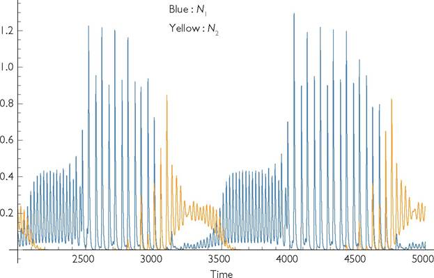
Fig. 8.6 The time course of consumer dynamics in a 2-consumer system with consumer 1 having seasonal variation in c and consumer 2 having no seasonal variation (γ1 = 0.9; γ2 = 0). The environmental period is q = 24. Both species have identical values of the other parameters, which are given in the legend of Figure 8.3. The dynamics are aperiodic.
8.2.6 A more complete description of seasonal interactions
The analysis thus far has not examined the quantitative nature of the interaction; how much does one consumer change in abundance with some change that only affects the other consumer? How much does abundance change (and in what direction) if the other consumer is removed? A related set of questions deals with the robustness of coexistence generated by seasonality when it occurs. In other words, how far can a fitness-related parameter in one species be changed without causing extinction of the other species (or of itself)? In the case of these unequal systems, how does the similarity in seasonal response curves affect the ability of species to coexist? Can species that are unable to coexist in completely symmetrical cases be made to coexist by giving one or the other an advantage or disadvantage? These questions all require numerical approaches, so there is only room for a few illustrative examples below.
The robustness of coexistence, when it occurs in the symmetrical system, can be measured by the maximum disadvantage in one species' fitness parameter(s) (or advantage in its competitor's parameter(s)) that allows both to persist. A convenient parameter in the models considered here (and in many natural systems) is the per capita death rate of one of the consumer species. Changing d, or any parameter that only affects the per capita growth rate of the focal species, is also the way that indirect interactions are traditionally measured (Yodzis 1988). In the traditional (aseason- al) MacArthur model, the change in population sizes of both species produced by a defined change in the mortality of one of them is independent of the current population sizes or mortality rates (provided the comparison involves no change in the number of consumers or resources). The next two figures show that this is not the case in the seasonal model considered here.
Figure 8.7 shows the impact of changing the mortality rate of consumer species 1 in the example of anti-synchronized species with variation in c(t). The parameters are as in Figure 8.3, with q = 60 and L = 30. Both consumers have an initial mortality of 0.2. Species 1 (blue dots) goes extinct when its mortality reaches 0.29, and species 2 (red dots) goes extinct when species 1's mortality drops to 0.07. Notice that both extinctions represent discontinuous changes in population size; in both cases, the drop is larger than the difference between the equilibrium size (when d1 = 0.2) and the population size for the mortality rate immediately lower than the extinction value (d1 = 0.08 for extinction of species 2 and d1 = 0.28 for extinction of species 1). Near the original equilibrium, the effects of mortality are very small, and consumer 2's abundance actually decreases as consumer 1's mortality increases for initial mortalities between d1 = 0.18 through and including d1 = 0.24. Thus, for close to 1/3 of the possible range of mortalities, species 1 has a positive effect on species 2, according to the standard (Yodzis 1988) method of measuring indirect effects. In fact, d1 = 0.27 is the first mortality rate greater than the equilibrium of 0.2 that produces a consumer 2 population greater than its original equilibrium value (at d1 = d2 = 0.2). At d1 = 0.25 the two consumers have nearly identical mean population sizes. Increasing the mortality of one species does not have a large effect on the abundance of the other until the mortality of the manipulated species is close to that which causes its
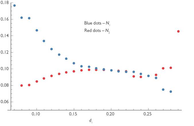
Fig. 8.7 'The response of mean consumer abundances to increased or decreased per capita mortality of consumer 1. The system is based on the parameters given in Figure 8.3 with q = 60, and both consumers having the same parameters except that consumer 2’s c value is lagged by 30 time units.
own extinction. Mortalities of 0.25 through 0.28 are associated with very long period or irregular population fluctuations.
The range of mortality rates allowing coexistence for the system in Figure 8.7 is relatively large. A good comparison case is an analogous non-seasonal system with standard resource partitioning. Here the resource population consists of two species, each with half the equilibrium abundance of the preceding case (due to a k value twice as large). The two consumers are assumed to have opposite specializations on the two resources, but have the same mean C of 1; i.e. a lower value of Cl and a higher value of Ch where Cl + Ch = 2. Moderate specialization with Cl = 0.8 and Ch = 1.2 yields coexistence for d1 = 0.14 through 0.29, a range approximately 3/4 that in Figure 8.7. Greater partitioning with Cl = 0.7 and Ch = 1.3 yields coexistence for d1 = 0.12 through 0.36, which is 6/5 times the range in Figure 8.7. The extreme values of mortality that limit coexistence in this non-seasonal model correspond to cases in which the lower-d species causes extinction of one of the resources, and this produces a discontinuous change in the abundance of the surviving consumer species.
Another example of responses to mortality (i.e., ‘interaction shape’) is provided by a seasonal MacArthur model with a single resource, anti-synchronized consumers, and a period length of q = 60. The other initial parameters are r = 1; k = 0.01, m = 0.001, γ1 = γ2 = 1; Ci = C2 = 0.25; Bi = B2 = 0.2; d1 = d2 = 0.25. These parameters produce anti-synchronized dynamics of the two consumers with equal mean densities of 1.6928. Figure 8.8 shows how increasing the per capita mortality rate of species 1 alters the temporal mean abundances of both species. In Figure 8.8A, the mean abundance of consumer 1 is given by blue dots, and that of consumer 2 by black dots. Figure 8.8B shows the corresponding estimated competition coefficient at each mortality rate calculated from the ratio of the population change in the unmanipulated species to that in the manipulated one, whose death rate is increased to the next larger value. Most of the larger jumps in population sizes or the competition coefficient occur as a result of qualitative changes in the dynamics as the death rate of consumer 1 is increased. Exclusion of species 1 occurs when d1 reaches approximately 2.1. Positive values of the competition coefficient imply that the mean densities of both species change in the same direction in response to increased mortality of species 1; there are cases in which this involves increases in both, and others in which both decrease following higher mortality of consumer 1. The frequent competition coefficients that are much larger than 1 in absolute magnitude indicate a much greater effect of the parameter change of species 1 on the population size of its competitor than on its own population size. This occurs in spite of maximal temporal partitioning and equal mean values of all of the parameters.
If the system described in Figures 8.8A and 8.8B had a shorter period, q, the relationships would change considerably. The system only exhibits alternative exclusion for integer periods of 6 and smaller. The period-60 case illustrated in Figure 8.8 is thus well above the q = 7 required to produce coexistence. In general, the extent of competition decreases with longer periods. In spite of the long periods, the density of each species alone (4.489) is much greater than the sum of the two densities when they occur together with equal mortalities (3.384). This increase is greater than the largest effect possible under an LV model of two exploitative competitors.
Another potential consequence of seasonal variation in systems with equal mean parameter values is the presence of alternative coexistence attractors having unequal mean abundances of the two consumers. In these cases, the effect of one species on another (as measured by the response to altered mortality of the first) differs greatly depending on which of the alternative states is originally occupied. An example of such a scenario based on the MacArthur system is exhibited by the following parameter set: {r = 1, k = 0.01, γ1 = γ2 = 1, C1 = C2 = 0.25, B1 = B2 = 0.1, d1 = d2 = 0.25, m = 0.001, q = 7, L = 3.5}. This has two alternative long-period cycles in which the mean abundance of one consumer is approximately three times greater than that of the other. Initial conditions determine which is more abundant. Not surprisingly, any quantitative measure of the interaction will depend on what attractor characterizes the initial state, and whether the perturbation used to measure the interaction shifts the system to the other attractor.
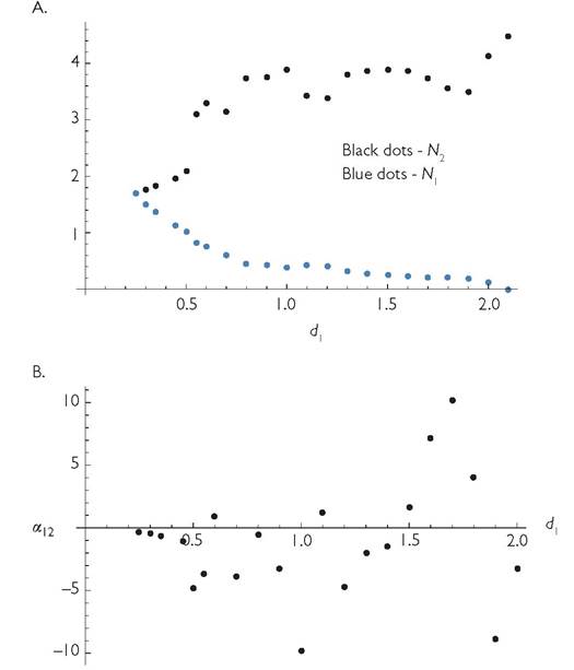
Fig. 8.8 Panel A. 'The mean population sizes of two competing consumers as a function of the mortality rate of consumer 1 for a MacArthur system in which the common parameter values are: q = 60; L = 30; r = 1; k = 0.01; m = 0.001; γ1 = γ2 = 1; C1 = C2 = 0.25; B1= B2 = 0.2; d2 = 0.25. The initial mortality of consumer 1 is identical to that of species 2 (d1 = 0.25), and the graph shows the changes in both species as the mortality rate of consumer 1 is increased.
Panel B. The competition coefficient based on the changes shown in panel A; the method of calculation is described in the text.
8.2.7 Seasonality resource conversion efficiency, b
The attack rate, c, has been assumed to be the seasonally changing characteristic in most previous analyses of seasonally varying competition (Abrams 1984a, Loreau 1992, Li and Chesson 2016). An alternative is that the consumers’ resource conversion efficiencies, b, vary seasonally. Variation in b differs from variation in c qualitatively,
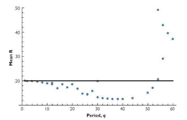
Fig. 8.9 'The mean resource density as a function of period length for a system with a single consumer species. The parameters are as in Figure 8.3, but the variation is in the conversion efficiency, b.
in that the variable factor in this case only has a direct effect on the consumer’s dynamics. Assume b varies periodically in a single-consumer system that has the same mean parameter values as in Figure 8.3. This produces mean resource densities for a range of period lengths, q, given in Figure 8.9. These results show that the single-consumer system undergoes a sequence of changes in dynamics as the environmental period is lengthened.
In the single-consumer system, the lowest period that has an attractor with a mean resource density greater than the constant equilibrium value of 20 is q = 54. Thus periods < 54 produce alternative exclusion. Periods above 60 (not shown) also had a single attractor characterized by a mean resource density significantly above 20 (q = 120 was the longest period that was examined). The results for competition between anti-synchronized consumers over a wide range of periods are summarized in Table 8.3. Alternative exclusion happens over a broad range of environmental periods; coexistence is not a possible outcome until q ≥ 54. All periods above 54 exhibited coexistence; q = 54 was the only case examined where coexistence, exclusion of consumer 1, and exclusion of consumer 2 were all possible outcomes.
The main differences between competition with b-variation in this example and the corresponding system having variation in c are: (1) alternative coexistence and exclusion outcomes for a particular system are less common; and (2) there is only a single transition between the two types of outcome as the period length is changed in a directional manner; alternative exclusion occurs for q < 54, and coexistence for q > 54. These two qualitative differences have been observed with periodic b for several other parameter sets, but their generality remains unknown. The system described
Table 8.3 Outcomes of 2-consumer competition with periodic variation in b. 'The parameters in eqs (8.1) are {r = 0.25, k = 0.00125, γ1 = 0.9, γ2 = 0.9, Ci = 1, C2 = 1, B1 = 0.01, B2 = 0.01, d1 =0.2, d2 = 0.2, m = 0.001}
| Period, q | Outcome | Population period | Population dynamics* |
| 12 or less | altern. exclusion | q | simple cycle |
| 14 | altern. exclusion | 2q | simple cycle |
| 16 | altern. exclusion | aperiodic | chaos |
| 18 | altern. exclusion | 12q | 4-cycle |
| 20 | altern. exclusion | 2q | simple-cycle |
| 22 | altern. exclusion | aperiodic | chaos |
| 24 | altern. exclusion | 4q | 2-cycle |
| 26-54 | altern. exclusion | q | simple cycle |
| 54 alt. | coexistence | aperiodic | chaos |
| 56, 58 | coexistence | aperiodic | chaos |
| 60 | coexistence | 6q | alternative 6-cycles |
| 70 | coexistence | 3q | alternative 4-cycles |
| 80 | coexistence | aperiodic | irregular |
| 90 | coexistence | aperiodic | irregular |
| 100 | coexistence | q | simple cycle |
| 120 | coexistence | q | simple cycle |
* Dynamics are classified bythe number of distinct population peaks of the resource during the course of a single cycle
in Table 8.3, and most other cases of b-variation examined also had mutual exclusion outcomes at low q for parameter sets where exclusion was a possibility.
8.2.7 A 3-consumer system with variation in c
The analysis has thus far only considered two consumers. A wide range of outcomes also occurs in the case of three temporally displaced, but otherwise equal competitors. Table 8.4 is based on the same mean parameter values as Figure 8.3, except that there are three competitors, with the second and third having lags of 1/3 and 2/3 of a period relative to consumer 1.
The population trajectories for one of the three attractors for q = 300 are illustrated in Figure 8.10. The other two attractors are identical in form and in their temporal order of species dominance, but differ in which of the consumers is identified with a particular dynamic role. Each line in the figure may characterize any one of the three species. The species identities associated with the three trajectories are determined by initial conditions. Note that the attractor is either aperiodic or has a cycle with a very long period.
Table 8.4 Competitive outcomes with three consumers and variation in c. The species have c-curves that are offset by 120 degrees (i.e., q/3). Other parameters are given in the text
| Period, q | Outcome | Population period | Population dynamics |
| 12 or less | altern. exclusion | q | simple cycle |
| 13 | altern. exclusion | 2q | two cycle |
| 14,15 | altern. exclusion | 2q | asymm. cycle |
| 16 | altern. exclusion | irregular, then 2q | asymm. cycle |
| 17 | altern. exclusion | irregular, then 4q | 2-cycle |
(All of above outcomes are preceded by ever-lengthening periods of dominance by different species with ever-decreasing population minima for the other two species; each species is largely replaced by the species having the next earlier peak in c(t))
| 18 | coexistence | irregular | bgcolor=white>chaos or very long cycle|
| 20 | coexistence | irregular | chaotic; varying dominance times |
| 22 | coexistence | irregular | chaotic; lengthening dom. times |
| 24 | coexistence | irregular | chaotic; order of dominance shifts |
| 28 | coexistence | irregular | irregular dominance intervals |
| 30 | coexistence | irregular | chaos-lengthening dominance |
| 35, 40, 50 | altern. exclusion | q | asymm. cycle |
| 60 | coexistence | q(short term) | long periods; altern. dominance |
| 70 | coexistence | 5q | 4-cycle; earlier replaces later |
| 80 | coexistence | 11q | 16-cycle; earlier replaces later |
| 90, | coexistence | 2q | simple cycles; earlier replaces later |
| 120, 150 | coexistence | q | simple cycles; later replaces earlier |
| 300 | coexistence | 4q | three complex cycles that differ only in species identities |
| * ‘altern. exclusion' means any one of the three species | can be the one that persists. | ||
In summary of the Table 8.4 example, coexistence of two or three species is impossible for short seasonal period lengths (q < 18; equivalent to slow population dynamics), and for a range of intermediate period lengths that includes the range of q between 35 and 50. Coexistence of all three is possible for all periods of 60 and above, as well as some more limited range of period lengths from approximately 18 to approximately 30. Forverylongperiods (e.g., q = 300; Figure 8.10) each consumer species undergoes several local peaks in abundance during its period of dominance, but each species has a different pattern of variation. The order of dominance of the coexisting species at periods of 120 and above corresponds to the temporal order of their lags (1 replaced by 2, 2 by 3, and 3 by 1). There are three distinct trajectories over time, with each species capable of exhibiting any trajectory. Seasonal periods significantly longer than q = 300 were not explored systematically.
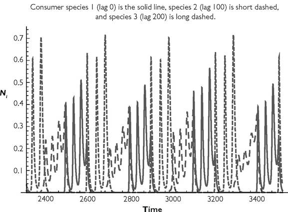
Fig. 8.10 The dynamics of a 3-competitor system with seasonality in attack rates. Here, q = 300, and consumers 2 and 3 have lags of 100 and 200 time units in their attack rates relative to consumer 1. The parameter values are given in the text.
8.2.9 A 2-resource system with temporal and non-temporal partitioning
The invasion curves shown early in this analysis (Figures 8.2A, B) suggest that the disadvantage to a rare invader with a lag is maximal for intermediate lags between 0 and 180 degrees. Given the symmetry of the system and the variation, the same applies to the effects (often an advantage for the invader) of lags between 180 and 360 degrees (q/2 - q). This should imply that, if the aseasonal system is characterized by coexistence due to resource partitioning or direct negative self-effects, coexistence in the seasonal system will occur more often when the two consumers have either very similar or very different patterns of temporal variation.
Introducing a second resource makes it possible to examine the impact of seasonal variation in systems that have partitioning by resource type. The example from Figure 8.3 may be converted into an equivalent 2-resource model by introducing a second resource, with the capture rate constants of consumer i on resource j denoted Cij. The mean of the two Cij values of each consumer is equal to the Ci value used in Figure 8.3. The two r values are the same as those in Figure 8.3, and the k value of each resource is multiplied by a factor of 2 to maintain the same equilibrium total resource population in the absence of consumption. When the B and d parameters are each equal for the two consumers, the dynamics of each consumer and the summed resource populations are identical to those in the single-resource system of Figure 8.3.
Table 8.5 Lags producing one or more outcomes of coexistence for a 2-resource system based on the Figure 8.3 example with period q = 36
Overlap*
| 0.9231 | Low L coexistence | Low L coexistence or exclusion |
| 0 ≤ L ≤ 3.65 | 3.56 < L ≤ 3.65 | |
| Medium L coexistence | Medium L coexistence or exclusion | |
| 16.6 < L < 19.4 | 15.9 ≤ L ≤ 16.6 and 19.4 ≤ L ≤ 21.1 | |
| High L coexistence | High L coexistence or exclusion | |
| 32.45 ≤ L ≤ 36 | 32.33 < L ≤ 32.44 | |
| 0.8 | Low L coexistence | Low L coexistence or exclusion |
| 0 ≤ L ≤ 6.46 | 6.47 ≤ L ≤ 6.53 | |
| Medium L coexistence | ||
| 12.41 ≤ L≤ 23.59 | ||
| High L coexistence | ||
| 29.54 ≤ L≤ 36 | ||
| 0.72414 | Coexistence for all lags |
* Calculated based on the MacArthur formula; see text
Resource partitioning maybe introduced by allowing Ci1 and Ci2 to differ from each other. Table 8.5 gives the ranges of lags L that permit coexistence of two consumers in systems having three different levels of resource partitioning, determined by the Cij. The table considers low resource partitioning (Cii = 1.2; Cj = 0.8; MacArthur α = 0.9231) and two higher levels of partitioning (Cii = 1.333; Cj = 0.6667; MacArthur α = 0.8; and Cii = 1.4; Cj = 0.6; MacArthur α = 0.72414). The table lists the lags that allow coexistence of the two consumers. Values of L close to the limits of coexistence are in some cases characterized by alternative outcomes of exclusion of the disfavoured species or coexistence. The disfavoured species is the lagged one for L < 18, and the non-lagged species when L > 18. For all lags other than L = 18, the abundances are unequal. Recall that in the corresponding system with one resource and a lag of exactly q/2, coexistence is impossible for q between 30 and 35, while both coexistence and exclusion of either species were possible for 36 < q < 60.
8.3
More on the topic A modelling framework and a seasonal MacArthur system:
- Developing green manufacturing framework through reverse logistics using system dynamics simulation
- 3.4 MacArthur’s connection of LV to consumer-resource models
- Modelling Past Rural Environment-Society Systems
- Seasonal Patterns of Trading Activity
- Why the Lotka-Volterra and MacArthur models are insufficient
- Seasonal changes in aquatic environments are associated with changes in water temperature and density
- Differences in nonlinearity with seasonal resource growth
- Agriculture-based Seasonal Festivals
- Modelling Language Shift
- Competition in seasonal environments: temporal overlap
- Modelling Innovative Societies in Its Environment
- Chapter 6 Modelling Routeways in a Landscape of Esker and Bog
- Resource extinction and quasi-extinction in MacArthur’s model
- Modelling Environmentally-Constrained but Adaptable Society-Environment Systems
- Chapter 7 Modelling Cultural Shift: Application to Processes of Language Displacement
- CONCEPT 2.5 Seasonal and decadal climate variation are associated with changes in Earth's position relative to the sun and the strength of atmospheric pressure cells.
- Chapter 8 Pathways for Scale and Discipline Reconciliation: Current Socio-Ecological Modelling Methodologies to Explore and Reconstitute Human Prehistoric Dynamics