Differences in nonlinearity with seasonal resource growth
Variation is a pervasive feature of the natural world (Pimm 1991). A major source of such variation in consumer species is variation in one or more growth parameters of one or more of their resources.
In a system with a single resource, variation in resource growth will only affect the consumer species differently if they have different shapes of their combined functional-numerical response or if the consumers also have temporal variation in their resource uptake or conversion rate parameters. To allow coexistence of two consumer species on a single resource, the consumer that is harmed to a greater extent by the fluctuations—i.e. the one with a more strongly saturating response—must also increase those fluctuations (or increase them to a greater extent).Abrams (2004b) examined competition using a number of simple 2-consumer-1- resource models with different types of variability in the resource growth rate. Abiotic as well as biotic resource growth models were explored in a setting where one consumer had a linear functional response and the second had a type II response. The models considered here are very similar, but they allow both species to have type II responses, and add the possibility that one or more of the consumer death rates vary sinusoidally. Consumer mortality rate variation is not considered until Section 9.4, and the analysis in both sections will be limited to logistic resource growth with an added immigration rate, m. The dynamics are given by:
As in Chapter 8, the parameters γi (0 ≤ γi ≤1) measure the amplitude of the sinusoidal variation, and the parameter q is the period length. Models with sufficiently low handling times do not allow sustained population cycles (or coexistence) in the absence of a temporally variable parameter.
If one consumer is characterized by Ch(r∕k) >1, then a sufficiently low mortality rate of that consumer will produce cycles in the absence of environmental variation (assuming immigration, m, is also very small). Abrams (2004b) showed that sinusoidal variation in the resource’s maximum per capita growth rate, r, could allow coexistence on a single resource type in a variety of 2-consumer models. That work showed that abiotic resource growth implied a significantly lower ability of resource-driven cycles to allow coexistence on a single resource than was true of biotic resources. Variable biotic growth of resources frequently produced a wide coexistence bandwidth, but a sufficiently short period, q, produced bandwidths close to zero.Although Abrams (2004b) stressed coexistence outcomes, the difference in the linearity of two consumers’ per capita growth rates is not sufficient to produce coexistence in all 2-consumer-1-resource systems having environmentally driven variation in resource growth rate, and may even prevent coexistence (as is shown below). In addition, models with variable resource growth can produce alternative outcomes that depend on starting conditions. As in the systems explored in Chapter 8 (where species did not differ in functional or numerical response shape), there may be an inherent periodicity in the dynamics of the underlying deterministic system, which interacts with the variation in resource growth rate to produce complicated dynamics. This leads to the possibility that the initial abundances determine whether two consumers coexist or not. Initial abundances in other cases determine which of two distinct coexistence outcomes prevails.
A diversity of outcomes for particular parameter sets characterizes a system that was the subject of Figure 4 in the Abrams (2004b) analysis. That figure examined the coexistence bandwidth for a system with a single logistic resource. The nonlinear consumer had a handling time that implied an approximate 90% reduction in the consumer’s per capita capture rate when the resource was at carrying capacity (relative to when the resource was rare).
The results in Abrams (2004b) suggested that all periods of variation produced a significant coexistence bandwidth. Those results also suggested that for the consumer 1 parameters assumed, only three qualitatively different outcomes were possible for different per capita mortality rates of consumer 2. These were: exclusion of 1 by 2 from all starting conditions at low d2; coexistence for a range of intermediate d2; and exclusion of consumer 2 by consumer 1 at sufficiently high d2. I was unable to replicate some parts of that figure in a recent reanalysis. In fact, this example has cases with coexistence and exclusion attractors for the same parameter set, and cases in which each consumer could exclude the other (alternative exclusion). Although the model in Abrams (2004b) lacked the low-level immigration into the resource population that are present in eqs (9.1), most of the differing results appear to be due to simulations that were not run long enough and a failure to look for alternative attractors. The results of a more accurate and more complete set of simulations for a small number of period lengths q are provided in Table 9.1.Table 9.1 Resource growth period length and consumer competition outcome; nonlinear functional response (eqs (9.1) with h2 = 0)
| Period q | Outcomes | Parameter range(s) |
| No variation | Exclusion of sp. 1 | d2 0.507 |
| 5 | Exclusion of sp. 1 | d2 0.508 |
| 10 | Exclusion of sp. 1 | d2 < 0.354 |
| Excl. of 1 or quasi-excl. of 2 | 0.354 < d2< 0.391 | |
| Exclusion of sp. 1 or sp. 2 | 0.391 < d2 < 0.399 | |
| Coex. or exclusion of sp. 2 | 0.399 < d2 < 0.421 | |
| Exclusion of sp. 2 | d2 > 0.421 | |
| 15 | Exclusion of sp. 1 | d2 < 0.467 |
| Exclusion of sp. 1 or sp. 2 | 0.467 < d2 < 0.502 | |
| Coex. or exclusion of sp. 2 | 0.502 < d2 < 0.539 | |
| Exclusion of sp. 2 | d2 > 0.539 | |
| 20 | Exclusion of sp. 1 | d2 < 0.457 |
| Coexistence | 0.457 < d2 < 0.579 | |
| Coex. or exclusion of sp. 2 | 0.579 < d2 < 0.606 | |
| Exclusion of sp. 2 | d2 > 0.606 | |
| 30 | Exclusion of sp. 1 | d2 < 0.340 |
| Coexistence | 0.340 < d2 < 0.695 | |
| Exclusion of sp. 2 | d2 > 0.695 | |
| 60 | Exclusion of sp. 1 | d2 < 0.270 |
| Coexistence | 0.270 < d2< 0.811 | |
| Exclusion of sp. 2 | d2 > 0.811 | |
| 100 | Exclusion of sp. 1 | d2 < 0.232 |
| Coexistence | 0.232 < d2 < 0.860 | |
| Exclusion of sp. 2 | d2 > 0.860 |
All of the systems considered above are characterized bythese parameters in eqs. (9.1): b1 = b2 = C1 = C2 = 1; h1 = 10; h2 =0; r = k = 1; d1 = 0.06. The amplitude of the variation in r is 1.
* quasi-exclusion denotes persistence with a mean density at least two orders of magnitude less than that of the dominant species
The system with no intrinsic resource variation allows coexistence via the Armstrong-McGehee mechanism; the nonlinear consumer generates cycles over a range of d2 values that spans more than a third (35.7%) of the total range of d2 values that allow consumer 2 to persist in the absence of consumer 1 (see Table 9.1). The minimum of d2 = 0.150 for coexistence is because lower mortalities imply that consumer species 2 can persist at a lower constant resource density than can consumer 1, and will therefore exclude it. Intrinsic variation of the resource growth rate with the relatively short period of q = 5 contracts, rather than expands, the range of mortalities of species 2 that allow coexistence. However that value of q is sufficient to produce enough resource variation that it reduces the per capita rate of increase of the nonlinear consumer 1 even when both consumers are very rare. Because of its rarity, the linear consumer 2 has little influence on the resource dynamics at the upper end of the coexistence range for d2. Here, the long-period consumer resource cycles, similar to what would occur with no variation in resource growth, dominate the dynamics. Thus the upper limit of d2 is not changed greatly by the presence of variable resource growth.
The dynamics become more complicated when q = 10. This period makes it possible for the resource growth cycles to suppress the interaction-driven cycles caused by consumer 1 under some circumstances. This results in the possibility of two or three different outcomes for a given system, depending on initial conditions (i.e., initial abundances and the initial phase in the resource growth cycle). A period of q =10 results in a significant range of mortalities of the linear species (0.354 < d2 < 0.391) that are characterized by coexistence, but at very low relative abundance of consumer 2.
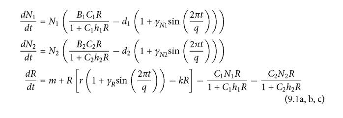
At slightly higher d2 there are only alternative exclusion outcomes. Figure 9.1 illustrates these alternatives for d2 = 0.395, and shows their associated different resource dynamics. Dominance by either consumer produces resource dynamics that favour it over its competitor. For a wide range of slightly higher mortalities of consumer 2, the alternatives are either coexistence or exclusion of 2. These alternatives are shown in Figure 9.2. If the species occupy the coexistence attractor at d2 = 0.420, the mean density of species 2 is approximately 61% that of species 1, but its equilibrium abundance drops to zero if d2 is raised marginally to 0.421.The range and nature of outcomes with a resource growth period of q = 15 is also complicated. For a significant range of intermediate d2 values (0.467-0.502), coexistence is impossible, and either consumer excludes the other, depending on initial densities. The next higher range of d2 (0.502-0.539) exhibits either coexistence of both species or exclusion of species 2. Still higher periods, q > 0.539, only produce exclusion of consumer 2. A resource growth cycle period of q = 20 allows coexistence over roughly 15% of the full range of mortalities that permit existence of species 2 in the absence of its competitor. However, a significant fraction of this range also has the alternative outcome of exclusion of species 2. The remainder of the periods explored in Table 9.1 (q = 30 and above) never resulted in alternative outcomes for any mortality rate. All of these longer periods produced the three outcomes of exclusion of 1 (at low d2), coexistence (at intermediate d2), and exclusion of species 2 (at high d2). The total coexistence bandwidth increases over this range of period lengths from q = 30 to q = 100. Longer periods increase the strength of intraspecific relative to interspecific competition by lengthening the stretches of time characterized by an advantage of one consumer over the other.
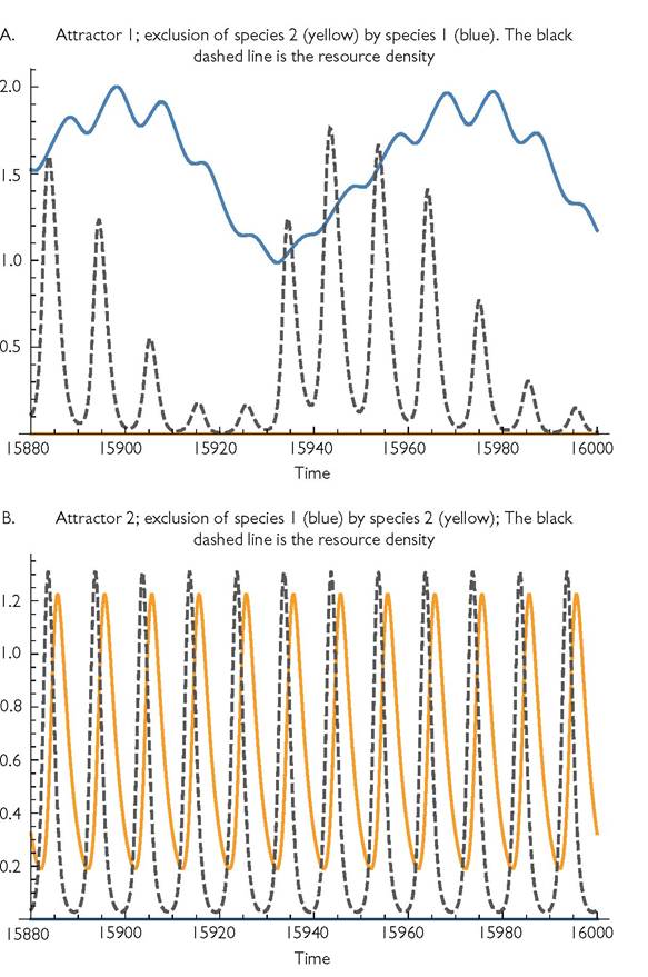
Fig. 9.1 Dynamics of consumer 1 and the resource, or consumer 2 and the resource for q = 10 in the Table 9.1 nonlinear functional response model with d2 = 0.395. These are alternative exclusion outcomes. In panel A, the nonlinear consumer 1 dominates the dynamics and produces irregular oscillations in population sizes with the larger amplitude fluctuations having a period greater than 80. The result is a low mean resource abundance that excludes consumer 2. If consumer 2 is initially sufficiently abundant the final dynamics are as shown in panel B. Here there is a simple period-10 cycle, with a high amplitude rapid fluctuation in resource abundance that excludes the nonlinear consumer 1.
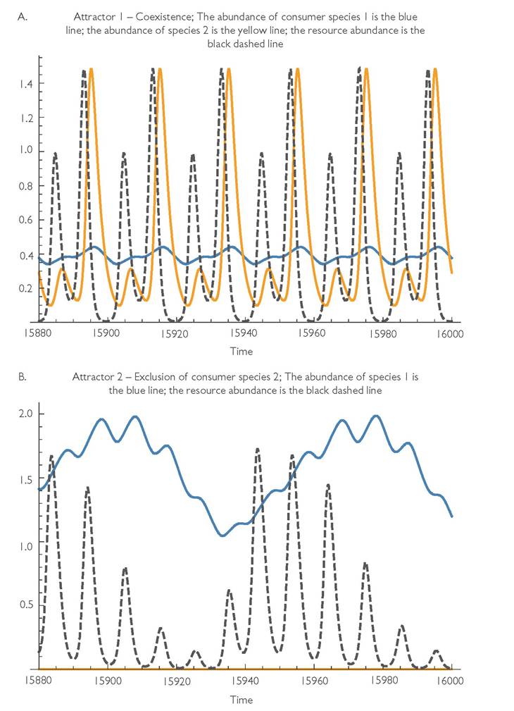
Fig. 9.2 The potential dynamics for the same Table 9.1 system with q = 10 illustrated in Figure 9.1, but with mortality increased by about 3.8% to d2 = 0.41. Rather than alternative exclusion outcomes, this system exhibits either coexistence or exclusion of species 2. The coexistence outcome shown in panel A has a period of 20, or twice the period of the resource growth rate variation.
In terms of classifying coexistence mechanisms, the Armstrong-McGehee system (with or without variation in resource growth) exhibits differences in the linearity of the functional responses, so it is a case of ‘relative nonlinearity’. However, it also exhibits periodic variation in the per capita intake rate of the nonlinear consumer on the resource, due to the cycles in resource abundance, which make the functional response more or less saturated at different points in time. This makes the ‘advantage’ in per capita growth rate switch periodically between the two consumer species. A similar variation in the relative attack rates (and thus relative per capita growth rates) of the two consumers in the systems considered in the previous chapter is what allows coexistence for some parameter values in that system. However, the systems in Chapter 8 lack any differences involving the nonlinearity of consumer functions. Both the systems considered immediately above and those in Chapter 8 involve periodic shifts in competitive advantage. Thus, it is unclear whether the ‘mechanisms producing competition’ are truly distinct in these two cases.
There are several values of q with parameter ranges for which each competitor is able to prevent the other from increasing from low abundance. In all of these cases coexistence would also be impossible if the system (eqs (9.1)) were modified so that each consumer had a very small direct negative effect on its per capita growth rate. This means that environmental variation in resource growth is capable of preventing coexistence in cases where it would otherwise be possible, for at least some ranges of both species’ mortality rates.
The example illustrated in Figures 9.1 and 9.2 is based on the scaled parameter values used in Abrams (2004b). There has not yet been a systematic exploration of the model behaviours across all potentially plausible parameter combinations in the system with variation in resource growth. However, a wide range of other parameter values exhibit alternative attractors involving coexistence and exclusion. Figures 9.3 and 9.4 illustrate two such cases for two systems with parameter values more similar to those employed in the main examples used in Chapter 8 (which, in turn, are similar to those adopted in Li and Chesson (2016)).
It is true that a difference in the linearity of at least one fitness component (the functional responses of the consumer species) in the Armstrong-McGehee model is an essential component of the ‘coexistence mechanism’. However, it is not sufficient that there be a difference in nonlinearity for coexistence to be possible for some combinations of values of the consumer mortality rates. Nor do all differences in nonlinearity between two consumers allow coexistence for some values of the mortality rates. Moreover, the nature of interspecific effects and the coexistence bandwidth can differ greatly, depending on the mechanistic basis of the interaction. This may be illustrated with a few examples employing often used, but seldom combined, model components. It should be noted that the definition of ‘relative nonlinearity’ has evolved since Chesson (1994) first defined it (e.g. Kang and Chesson 2010), and the latter paper acknowledges that it may not always favour coexistence. There is still not a clear verbal definition of the mechanism labelled as ‘relative nonlinearity’.
Coexistence in the system described above cannot be attributed solely to differences in the shapes of the consumer growth functions. This is because the difference in nonlinearity is due to differences in the functional response shapes.
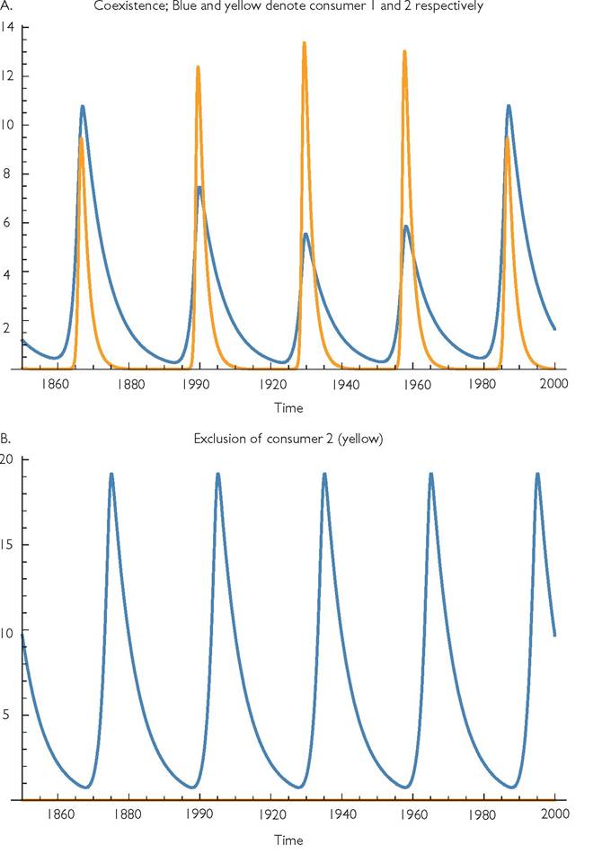
Fig. 9.3 Alternative attractors for eqs (9.1) with a logistic resource, variable resource growth, and parameter values: r = 1, k = 0.01, C1 = 0.25, C2 = 0.25, h1 = 0.1, B1 = B2 = 0.1, d1 = 0.15, d2 = 0.5, m = 0.0001, q = 30, and γκ = 0.75. Panel A has consumer coexistence with cycles of period 120 (= 4q). The mean abundances of N1, N2, and R are: 2.2654, 1.2807, and 20. Panel B has population cycles matching the environmental period (q = 30) and mean abundances N1, N2, and R are respectively 5.8133, 0, and 19.191.
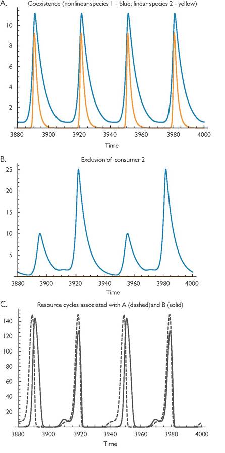
Fig. 9.4 Alternative attractors for eqs (9.1) with a logistic resource, and parameter values: r = 1, k = 0.01, C1 = 0.25, C2 = 0.25, h1 = 0.1, h2 = 0, B1 = B2 = 0.1, d1 = 0.175, d2 = 0.51, m = 0.0001, q = 15, and = 0.75. Panel A shows consumer densities for the coexistence attractor, and panel B shows the abundance of consumer 1 for the exclusion attractor. Panel C shows the resource abundances corresponding to panels A and B, with the solid line corresponding to panel B.
The potential instability of a system that lacks variable parameters is due to the impact of the consumer’s nonlinear functional response on the resource dynamics (e.g., May 1973). A sufficiently saturating response results in a net positive effect of increased resource abundance on the resource per capita growth rate near the equilibrium point in unstable systems. Thus, it is of interest to determine whether differences in the nonlinearity of consumer growth per se are able to generate coexistence of two consumers in the absence of direct effects of that nonlinearity on the stability of resource dynamics.
One can explore the role of differences in consumer nonlinearity per se by analysing a system in which one consumer has a nonlinear numerical response, the other has a linear numerical response, and both have linear functional responses. The shapes of numerical responses have largely escaped empirical study, but it is well known that physical constraints place upper limits on birth rates, so saturation of numerical responses is inevitable. The nonlinearity in the numerical response can bring about coexistence if there are cycles driven by temporal variation in some other parameter. The nonlinear (saturating) species is more adversely affected by variation in resource density. Thus, if the nonlinear species is able to increase when rare, and it also causes greater amplitude cycles in resource abundance when it is common, both species should be able to persist. The next section considers variation in the resource per capita growth rate, to make it as similar as possible to the systems with a nonlinear functional response discussed above and in Abrams (2004b).
9.4