Differences in the nonlinearity of numerical responses
Most saturating functional responses are capable of generating cycles in most models with purely biotic resource growth. This is not true for a saturating numerical response in which consumer growth rate is solely a function of resource abundance.
The form of the numerical response has received remarkably little empirical attention (as noted in Getz (1993) and Abrams (1997)). However, saturation should be a general property due to the restrictions body size and other factors place on maximum reproductive rate. A simple form for such a model is given below, for a system where each species has a linear functional response but species one has a nonlinear numerical response with the same (Michaelis-Menten) shape as Holling’s type II disc equation. The resource may have temporal variation in its maximum per capita growth parameter, r. The resulting model has the form: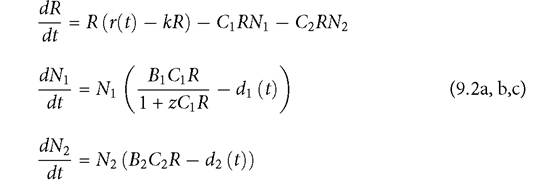
The parameter z plays the same role in determining the per capita growth rate function for consumer 1 as does the ‘handling time' in a type II functional response (h in eqs (9.1)). However, here z reflects limitations on the growth and/or birth rate of the species rather than limitation on time available for searching for resources. A positive value of z cannot bring about coexistence of the two consumers in the absence of some other factor that generates sustained cycles. In eqs (9.2), there are three potentially time-dependent parameters, which will be examined below. The variation in each time-dependent parameter is assumed not to affect the mean value of the parameter. The simulations described below impose variation using the same multiplicative sinusoidal function with a mean value of 1 given explicitly in eqs (9.1). If all of the functions of time in eqs (9.2) were constants, the system could only have a stable equilibrium with a single consumer present (ignoring the theoretical possibility of a neutral line of equilibria).
The consumer characterized by a lower equilibrium resource density would exclude the other.The first case considered here is variation in the resource per capita growth rate. Here the parameter r changes sinusoidally and this variation in resource growth leads to sustained cycles in the abundances of all three species. The convex shape of consumer 1’s growth function makes it more likely that any type of variation will increase both the mean resource abundance required for the consumer to increase when rare, as well as the long-term mean resource abundance when the nonlinear consumer is present alone. Variation in either or both consumer death rates also cause sustained density fluctuations; their effects on the interaction between consumers will be considered later, in Section 9.5.
The parameters used here are equivalent to those used in the main example of eqs (9.1) discussed in Section 9.3. These are: B1 = B2 = C1 = C2 = 1; z = 10; r = k = 1; d1 = 0.06. The amplitude of the cycle in r is assumed to have its maximum value, implying sinusoidal variation with a minimum r(t) = 0 and a maximum r(t) = 2. In the system where consumer 1 has a nonlinear functional response (eqs (9.1)) and no variation in r, these parameter values imply large amplitude consumer-resource cycles and a coexistence bandwidth (range of d2) of approximately 0.357. This compares with the maximum range of 1.0 for d2 that allows existence of the linear species in the absence of competition. On the other hand, a difference in the nonlinearity of the two numerical responses never allows coexistence; the only possibilities in this example are exclusion of consumer 2 for d2 > 0.15 and exclusion of consumer 1 for d2 < 0.15.
Table 9.2 describes the outcomes of competition in a system that is identical to that of Table 9.1 except that it is the numerical rather than the functional response of consumer 1 that is nonlinear.
Table 9.2 shows that coexistence is impossible for the three lowest environmental periods studied; q = 5,10, or 15. Periods of 10 and 15 have a significant range of d2 values that produce exclusion of either species, roughly corresponding to initial abundances. (The ‘roughly’ arises from the influence of the initial direction of change in resource growth, which can reverse the relative population size during the initial time span.) If small magnitude direct negative effects of each consumer’s density on its own growth rate were added to eqs (9.2) this wouldTable 9.2 Resource growth period length and consumer competition outcome; nonlinear numerical response model (eqs. 9.2)
| Period q | Outcomes | Parameter range(s) |
| No variation | Exclusion of sp. 1 | d2 0.150 |
| 5 | Exclusion of sp. 1 | d2 0.182 |
| 10 | Exclusion of sp. 1 | d2 < 0.281 |
| Exclusion of sp. 1 or sp. 2 | 0.281 < d2 < 0.400 | |
| Exclusion of sp. 2 | d2 > 0.400 | |
| 15 | Exclusion of sp. 1 | d2 < 0.400 |
| Exclusion of sp. 1 or sp. 2 | 0.400 < d2 < 0.500 | |
| Exclusion of sp. 2 | d2 > 0.500 | |
| 20 | Exclusion of sp. 1 | d2 < 0.459 |
| Coexistence | 0.459 < d2 < 0.484 | |
| Coex. or exclusion of sp 2 | 0.484 < d2 < 0.529 | |
| Exclusion of sp. 2 | d2 >0.529 | |
| 30 | Exclusion of sp. 1 | d2 < 0.341 |
| Coexistence | 0.341 < d2 < 0.584 | |
| Coex. or exclusion of sp. 2 | 0.584 < d2 < 0.588 | |
| Exclusion of sp. 2 | d2 > 0.588 | |
| 60 | Exclusion of sp. 1 | d2 < 0.270 |
| Coexistence | 0.270 < d2 < 0.704 | |
| Exclusion of sp. 2 | d2 > 0.704 | |
| 100 | Exclusion of sp. 1 | d2 < 0.232 |
| Coexistence | 0.232 < d2 < 0.750 | |
| Exclusion of sp. 2 | d2 > 0.750 |
The parameters sharedwith the Table 9.1 model havevalues identical to those in Table 9.1;the one newparameter, z, has a value of 10.
allow coexistence for some range of relative mortality rates in this system without resource growth variation. However, coexistence would not occur (or the self-effects would have to be larger for it to occur) in cases with alternative exclusion outcomes. Thus, one can describe the effects of temporal variation as making coexistence more difficult. (As discussed in Chapter 10, this conclusion maybe reversed if the species occur in a spatially structured metapopulation.)
The nonlinear numerical response system with q = 20 has four categories of outcomes, including a relatively narrow range of d2 where coexistence of both species or exclusion of the linear species are alternatives.
The latter range of d2 is even narrower when q = 30. Periods of 60 and greater produce wide coexistence bandwidths, and no cases of alternative outcomes. The coexistence bandwidths are all somewhat smaller than those in the corresponding nonlinear functional response models.In summary of the results in Table 9.2, models with nonlinear numerical responses can exhibit coexistence on a single resource in environments with temporally variable resource growth. However, not all types of environmental variation in resource growth allow some coexistence, and variation with a relatively short environmental period can make coexistence more difficult or impossible. Although this is just one example, analysis of several other systems having large differences in numerical response shape also exhibited a wide range of potential effects of resource-driven variation.
9.5