Other types of environmental variation

Variation in the consumer mortality rates, which is included in eqs (9.1) and (9.2), can also affect coexistence. Such variation could occur in conjunction with nonlin­ear functional and/or numerical responses.

9.5.1 Nonlinear numerical responses

I begin by considering correlated mortality in both consumers in the numerical response model, eqs (9.2); both mortality rates vary between zero and twice their mean. The fact that the baseline consumer per capita mortality rates are low relative to the baseline resource per capita growth rate in the system considered here means that a longer period q is required to generate enough variation in resource abundance to have a significant effect on coexistence. Here, coexistence does not occur until q is considerably larger than 60, and the bandwidth is relatively narrow even for q = 100. When q = 60, not only is coexistence impossible for all d₂, but there are alternative exclusion outcomes for 0.335 < d₂ < 0.426. When q = 100, coexistence is the only out­come for the relatively narrow range of 0.351 < d₂ < 0.424.

The above comparison of single and dual consumer mortality variation can be understood qualitatively based on the general requirement that, in order for two species to coexist, at least one species must have some stabilizing process that decreas­es its relative competitive ability as its short-term mean abundance increases. If variable mortality is associated with the nonlinear consumer 1 in eqs (9.2), this will lead to greater resource fluctuations as its numbers increase, which will slow its growth and provide an opportunity for the linear species to coexist. Thus, variation in the mortality of consumer 1 produces a relatively wide coexistence bandwidth. This is reduced, but not eliminated by having mortality variation in the linear consumer as well. A numerically dominant linear species 2 produces large amplitude fluctuations in the resource that often give it the ability to exclude species 1.

9.5.2 Nonlinear functional responses

The comparable model with species 1 having a nonlinear functional response (Table 9.1 above) also yields somewhat different results when consumer mortal­ity variation is substituted for resource growth variation. In the absence of any environmentally caused cycles, consumer 1’s type II response implies a coexistence bandwidth for the linear species of d₂ = 0.15-0.507. Coexistence was examined in this variable consumer mortality model for periods of 15 and 30 to provide a com­parison with the case of variation in resource growth rates in Table 9.1. Somewhat less detailed results for q = 5 and q = 100 are given at the end of this section.

For q = 15, coexistence was always observed from d₂ = 0.286 through d₂ = 0.516. This compares to the much narrower bandwidth of 0.502 < d2 < 0.539 for the model considered earlier that only has variation in resource growth. Note that this coexistence attractor in the resource-variation model occurred in conjunction with an alternative attractor characterized by exclusion of consumer 2. Thus, vari­ation driven by fluctuations in both consumers’ mortalities was considerably more favourable for coexistence. However, this is largely because the smaller amplitude of consumer mortality cycles compared to resource growth cycles results in less interference of the environmentally driven cycles on the interaction-driven cycles.

If q = 30 for the consumer mortality variation, coexistence is possible from d₂ = 0.450 to d₂ = 0.535. Exclusion of consumer 1 always occurred below this range,

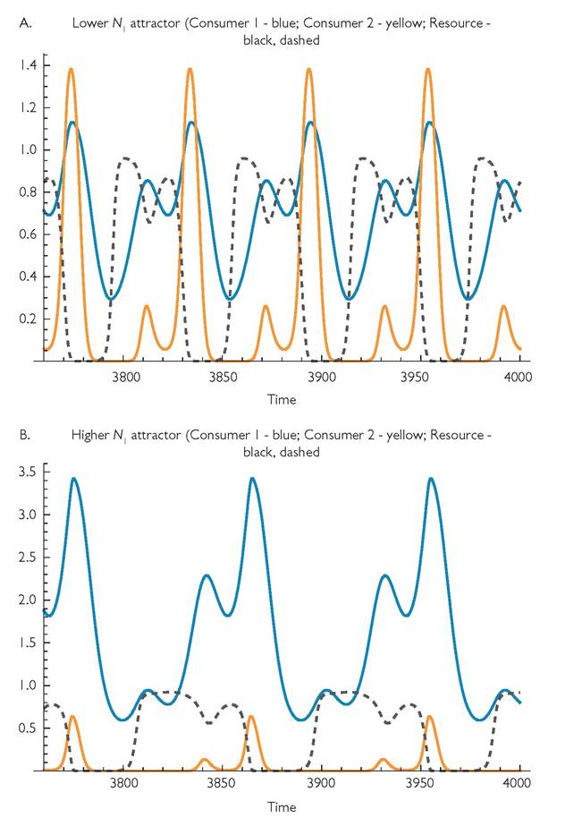
Fig. 9.5 An example of alternative coexistence outcomes that occur with the nonlinear func­tional response model having variation in both consumer mortality rates. The parameters are: r = 1; k = 1; Ci = 1, C₂ = 1; h_l = 10, h₂ = 0; B₁ = 1, B₂ = 1; d_i = 0.06, d₂ = 0.5; m = 0.0001; q = 30, γ_p1 = 1, γ_p2 = 1.

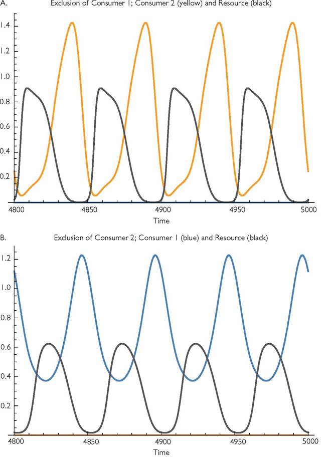
Fig. 9.6 'The alternative attractors for eqs (9.2) with variation in both consumers’ mortality rates. The parameters are: r = 1; k = 1; Ci = 1, C₂ = 1; h₁ = 10, h₂ = 0; Bi = 1, B₂ = 1; d₁ = 0.06, d₂ = 0.4; m = 0.0001; q = 50, γ_p1 = 1, γ_p2 = 1. Alternative exclusion outcomes exist for values of d₂ between 0.29625 and 0.545.

and exclusion of consumer 2 occurred above this range. This compares to the much wider range of mortalities allowing coexistence (0.340-0.697; see Table 9.1) in the comparable case of variation in resource growth rate with q = 30. This is again relat­ed to the fact that the environmentally caused variation is of greater amplitude in the case of resource growth variation than in the case of consumer mortality vari­ation. Unlike the preceding example (q = 15), q = 30 has a very positive effect on coexistence. The bandwidth noted above actually overstates the possibility of coex­istence in the consumer mortality variation model because one or more alternative attractors are found for a wide range of different mortalities in the q = 30 case. Most significant from the standpoint of coexistence is the fact that exclusion of species 2 by species 1 is a possible outcome for values of d₂ from 0.491 to the maximum of 0.536. Exclusion of species 1 by species 2 occurs as an alternative to coexistence for d₂ val­ues from 0.450 to 0.482. Thus, there is only a narrow range of mortalities of the linear species over which exclusion never occurs for any initial conditions (d₂ from 0.482 to 0.491). In addition, there are parameter ranges over which two different coexistence attractors exist, and parts of these ranges also allow a third (exclusion) attractor.

Very short periods (e.g. q = 5) in this consumer mortality variation model have relatively modest effects on coexistence bandwidth; the cycle driven by consumer 1 dominates the dynamics except when d₂ is low enough to greatly reduce the abundance of consumer 1. Moderately long periods are particularly likely to have alternative exclusion outcomes. Figure 9.6 shows the two exclusion outcomes that are possible if the parameter set described in the previous paragraph has q = 50 and d₂ = 0.4. This case allows alternative exclusion for a wide range of mortalities between d₂ = 0.296 and d₂ = 0.545. The alternatives illustrated in Figure 9.6 are character­ized by quite different mean resource abundances. Still longer periods (e.g. q = 100) have narrower coexistence bandwidths than in the otherwise comparable model with resource-growth driven rather than consumer mortality driven cycles. For the system considered in the previous paragraph coexistence occurs for d₂ between 0.36 and 0.59, which is roughly 1/3 the range for q = 100 under resource growth variation (see Table 9.1). This lower bandwidth is largely a consequence of the lower amplitudes of the resource fluctuations caused by consumer mortality rate variation compared to those caused by resource growth variation.

9.5.3 Remaining unknowns

This section definitely does not constitute an adequate analysis of the possible effects on competition between two consumers for a single resource with periodic varia­tion in consumer mortality rates. Many options regarding different amplitudes or phase shifts between consumers, or combinations of consumer- and resource-driven cycles remain to be explored.

Future work should examine: (i) various models of abiotic growth; (ii) biotic resource systems in which the resource’s own resource(s) are represented; (iii) models of combined abiotic and biotic growth; (iv) models with two or more potentially inter­acting resource species/types; and (v) models in which all species exhibit correlated seasonal variation in several parameters, as in most higher-latitude environments. The consequence of different dynamic rates of consumer and resource also needs more study. A wide variety of different functional response forms arise from adap­tive behaviour (Chapter 3), and some of these are likely to lead to different impacts on coexistence in variable environments.

9.6