Intraspecific competition

Chapter 2 noted that one of the earliest textbooks on population ecological theo­ry (Wilson and Bossert 1971) had discussed within-species competition under the heading of ‘density dependence’.

Intraspecific competition involves two or more resources in nearly all con­sumer species; true specialists are quite rare (Polis and Winemiller 1996). Thus, a basic understanding of intraspecific competition requires an understanding of the dynamics of systems with a single consumer of multiple resources. When the resources themselves are living species, this means that the process of apparent competition is inextricably linked to both intraspecific and interspecific competition.

5.2.1 The definition and mechanism of intraspecific competition

It is interesting that, like ‘interspecific competition’, the definitions of both ‘intraspe­cific competition' and ‘density dependence’ have long been the topics of debates that are still not settled. Regarding density dependence, Herrando-Perez et al. (2012) claim that most modern ecologists would agree on Murdoch and Walde’s (1989) def­inition of, ‘a dependence of per capita population growth rate on present and/or past population densities’. However, they go on to discuss a number of subsequent works by various authors who had different definitions. The definition of intraspe­cific competition used here is similar to the definition of interspecific competition proposed earlier; i.e., the effects of the abundance of a single species on its demo­graphic rates that are caused by the associated changes in the consumption rates of shared resources. Intraspecific interference effects are included, as they general­ly modify consumption of some resources used by other individuals, as well as by the focal individual.

Most of the criticisms of the LV competition model covered in previous chapters also apply to the logistic and other continuous-time single-variable models of single­consumer population dynamics. In both types of models the instantaneous growth rate is determined by the current population size. Like the MacArthur consumer­resource model, the logistic model for single-species population growth can be derived from a standard continuous-time consumer-resource model in which the resources are nutritionally substitutable, all resources have logistic growth, and none of the resources have the potential to be driven extinct by the interaction. The deriva­tion also requires that the consumer species have linear functional and numerical responses. These limitations mean that the use of the logistic model requires a rather unlikely set of assumptions to be an accurate representation, including the particular­ly troubling assumption that the logistic itself must apply to the growth of all of the resources.

The connection of density dependence to resources and the underlying mech­anisms of consumer-resource interactions has been recognized by many previous authors. For example, Begon et al.'s (2006, p. 411) textbook states: ‘[many studies]... have been concerned to detect “density dependent” processes, as if density itself is the cause of changes in birth rates and death rates in a population. But this will rarely (if ever) be the case: organisms do not detect and respond to the density of their populations. They usually respond to a shortage of resources..Even earli­er, Krebs (1995, 2002) and Sibly and Hone (2002) had argued that a mechanistic approach should replace the concept of density dependence. One of Krebs' (2002) arguments against simple density dependence is that previous attempts to quantify growth rate as a function of density have found that the relationship changes great­ly with time and with the location of the study.

The use of models of (consumer) population growth that include resource dynam­ics has a long history. A few of the many examples are Schoener (1973), Royama (1992), Rueffler et al. (2006b) and Johst et al. (2008). However, the relationship between consumers and resources is often ignored in applied areas of ecology, such as fishery regulation and conservation biology. It is common for fishery regulators to use simple models of single-species density-dependent growth to determine the abun­dance and harvest rate producing maximum sustainable yield, as well as the smallest population size that is consistent with minimal extinction risk. This can result in inappropriate regulations, as discussed in Matsuda and Abrams (2006, 2013).

Despite the opinions quoted above, many textbook treatments of intraspecific competition have continued to ignore the underlying consumer-resource interaction when discussing the topic of density-dependent growth.

5.2.2 Describing, measuring, and modelling intraspecific competition

The fundamental motivation for models of density dependence is to describe the relationship between population size and growth rate. However, this relationship is usually at least partly indirect, implying the presence of time lags. Adding or removing consumer individuals initiates a change in resource densities, but the consequences of such a change are not fully realized until resources respond and the system reaches a new equilibrium or dynamic attractor. By the time the resource response is mea­surable, the perturbed consumer population will likely have changed in size. Even if it were possible to maintain the consumer population at exactly its perturbed abun­dance by constant additions and removals, the effect of that population control often changes the pattern of change of the resource abundances to produce dynamics that would be impossible to achieve by altered values of neutral parameters. This is true, for example, in any system that would otherwise exhibit predator-prey cycles, as well as systems in which the flexibility of the manipulated species is required to maintain stability of the community in which it is embedded. As is true of interspecific compe­tition, the changes in both immediate dynamics and ultimate population size caused by a changed property of the focal consumer species differ depending on the nature of the dynamics of the consumer’s resources. The conclusion is that the dynamics of both consumer and resource must be modelled to describe density dependence.

Does the involvement of resources mean that the traditional view of a relationship between density and population growth must be discarded completely? The answer is no.

While the addition or removal of individuals (i.e., neutral parameters) are use­ful for quantifying interaction strength, the effects of other perturbations are also important if we are to fully understand intraspecific competition. Environmental changes often affect the nature of the consumer-resource interaction directly, for example, by altering the rate of capture of resources, and/or the effects of those consumption processes on demographic rates. Climate change is likely to affect activ­ity levels, and therefore resource uptake rates. This effect makes climate change a non-neutral perturbation, as it has an immediate effect on both consumer(s) and resource(s). An increase in its resource uptake rate can decrease a consumer pop­ulation in a much wider (and different) range of circumstances than those leading to a decreased population due to decreased mortality (Abrams 2002, 2003, 2004a).

Decreasing the abundance of resources directly by consumption is not the only mechanism by which consumer individuals can affect the resource intake of other members of their population. As in the case of interspecific competition, individ­uals of a single species can directly interfere with other individuals of that species, decreasing their rate of food consumption or imposing additional mortality. Preda­tors of the consumer species may have effects on the consumer’s resource uptake, so a quantitative description of intraspecific competition may often require consideration of higher trophic levels.

The only major mechanism that differs between intra- and interspecific compe­tition in animals is the (usually) negative impact of competition for mates and of mating itself, which are both (usually) interactions within a given species. These include energy expenditure and mortality on the part of females resisting mating, disease transmission, and direct negative effects of substances that are transferred by males in the process of successful mating (see Chapter 3 of Arnqvist and Rowe 2005). Males are also subject to mortality from other males while competing for females, and female-caused mortality due to cannibalism. Burke and Holwell (2021) describe an example of high female mortality as a result of violent male mating behaviour (which is, in part, a function of males trying to avoid cannibalism). This type of interaction could be a source of reduced population growth at higher densities. Mating-related mortality in males seems less likely to reduce population growth rates due to the abundance of mating opportunities for females of most species, once population size is simply moderate. However, the effects of male mortality are complicated, as reduced male numbers may also entail indirect positive effects on females due to reduced resource competition as a result of fewer males. For plants, higher popula­tion densities may attract more pollinators and/or reduce self-pollination, producing effects that may offset resource competition. The pollinator visits can be represented as resources, although their dynamics differ greatly from those of light and mineral nutrients. In any event, we know relatively little about the effects of such processes on population growth rates for most animals or plants, and distinguishing sexes is incon­sistent with the homogeneous-population approach used in most of this book, as well as most previous competition theory. Thus, sexual conflict will not be included explic­itly in the models discussed below, although it is one of many causes of intraspecific interference competition.

Even if the population-level consequences of sexual reproduction are ignored, the wide variety of potential resource dynamics and interference effects should have resulted in a comparably expansive variety of models of intraspecific competition.

Based on this, we should have expected a wide range of observed single-species population growth trajectories. The connection of consumer-resource models to density-dependent growth has been discussed occasionally over the last several decades (Schoener 1973; Schaffer 1981; Matessi and Gatto 1984; Abrams 2009b, c, d). Abrams (2009b, c, d) suggested that neither the logistic nor the somewhat more flex­ible theta-logistic (Pella and Tomlinson 1969; Gilpin and Ayala 1973; see eq. (5.1) below) is likely to provide a generally applicable model for the response of a con­sumer species to environmental change affecting population growth. Abrams (2009b) examined how the presence of multiple resources alters the form of intraspecif­ic competition, as reflected in the response of a consumer species' equilibrium or mean population density to changes in a neutral parameter. Abrams (2009a, b, c, d) and Abrams and Matsuda (2005) illustrate various implications of type II consumer functional responses for the viability of a logistic growth model as an approxima­tion to consumer dynamics. As in the 2-consumer case, nonlinear per capita growth of the resource, resource exclusion, and nonlinear consumer functional responses all produce nonlinear responses of population size to changes in neutral consumer parameters. They also produce the potential for discontinuous change in abundance with continuous change in a parameter (the latter being possible when at least some of the lower-level resources are self-reproducing).

Unlike traditional models of density dependence, resource-based models do not necessarily involve an immediate reduction in population growth rate following an increase in population size. The decrease happens after the additional consumers have significantly decreased the abundances of at least some of the resources. The one major set of exceptions to this generalization about delayed consequences is the category of effects produced by rapid (usually behavioural) change in either predators or prey in response to a change in predator abundance; prey may change activity to decrease their risk of predation in response to higher predator numbers. Predators may increase their foraging in the presence of others to ensure increased food intake before the local prey population is depleted. However, these behavioural effects are only one component of the feedback process by which current consumer abundance affects future consumer population growth. The feedback via altered abundance of resources always involves some delay. And because of predator-prey oscillations, even if they are damped and eventually disappear, there maybe prolonged and oscilla­tory changes in the abundances of consumers and resources following a perturbation to their abundances (see Figure 2.1). Such oscillations are less common, but they also occur in some systems with abiotic resources. Chapter 8 shows that these lagged responses can have a major effect on the nature of consumer-resource systems in seasonal environments.

The transient dynamics of models of a single consumer with one or more resources, and their responses to parameter perturbations in non-equilibrium sys­tems usually cannot be captured adequately with a model of direct density depen­dence (Reynolds and Brassil 2013; O'Dwyer 2018; see Chapter 8). It is nevertheless useful to determine how imposed mortality affects ultimate population size, as this reflects the action of the various processes that determine intraspecific competition.

It also provides a quantitative way to compare the responses of systems with two or more competing consumers to those with a single consumer species, as the mutual effects of altered mortality rates provide a standard measure of interspecific competition (Chapter 2).

For a consumer that uses biotic resources, analysing the interactions of those resource species with their own resources is often important for developing a model of the growth of the consumer population. The general need to consider lower-level entities may extend to two or more trophic levels below the focal species whose intraspecific competition is of interest. In any case, the prey's resources will display delayed responses to a change in prey abundance, contributing to a larger delay in the predator's response. This scenario calls for using a model with more trophic lev­els when the consumer species of interest is on the third or higher level. Having three or more dynamic entities opens up the possibility of more complex dynamics (Hast­ings and Powell 1991). Abrams and Roth (1994a, b) provide some examples of these dynamics in simple models where consumers on the top one or top two trophic levels have type II functional responses. The case when only the middle species has a type II response was considered in Abrams and Roth (1994a), who show that there are alternative attractors in the three-level system that have or lack cycles. With type II responses on both trophic levels, there are often alternative attractors (Abrams and Roth 1994b). Both types of three-level systems allow positive perturbations to growth of the bottom-level species to translate into decreases in the (mean) abundance of the top-level species, something that does not happen in simple continuous mod­els of density dependence with a strictly food-limited top species. These systems can even exhibit extinction of the top-level species as a result of increasing the carrying capacity of the bottom-level species. Hydra effects are often possible for the top-level consumer; its abundance decreases with lower mortality due to reduced production at lower levels in the food web. Loreau (2010) has presented the case for including all levels down to the abiotic resources used by plants. Most of the models considered below only include two trophic levels, so they understate the likelihood and mag­nitude of departures from traditional models of single-species density dependence. These traditional models are considered in the following section.

5.2.3 Models of density dependence

It was recognized long ago that the logistic growth model of Verhulst (1838) could not represent all forms of density dependence. The logistic model describes the con­sequences of intraspecific competition as a linear and immediate negative effect of abundance on per capita growth rate. The main alternative for many years was the ‘theta-logistic' model of Gilpin and Ayala (1973), which differs in allowing the effect of density to be a power function of abundance:

dN N√

* -^rN V ⅛1;

(5.1)

Sibly et al. (2005) analysed existing lengthy time series of population sizes in an attempt to estimate the value of the positive exponent, θ. Their methods were widely criticized (e.g., Ross 2006; Doncaster 2006, 2008; Getz and Lloyd-Smith 2006), and, in many cases, we do not know whether competitors or predators of the focal species had some influence on the time course of population change. Their data were typical­ly annual measurements of size, so it was actually a discrete version of eq. (5.1) that was used. Alternative nonlinear models of per capita growth were not considered. However, Sibly et al. (2006) argue for their original analysis, and their 2005 article remains the most comprehensive analysis of the form of single-species dynamics. The wide range of estimated exponents in that study is, at a minimum, strong evidence for great interspecific variation in the functional form of intraspecific competition. Figure 5.1 illustrates part of the range of shapes of the per capita growth rate function defined by eq. (5.1).

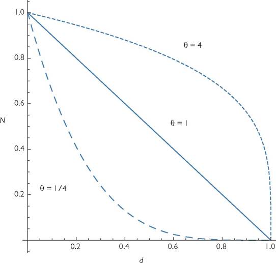
Fig. 5.1 The relationship between mortality and population size for the ‘theta-logistic’ model (eq. 5.1) under three different exponents.

In another review of empirical studies, Brook and Bradshaw (2006) analysed 1198 time series of abundances, and noted that clear evidence for any density dependence was lacking in approximately 25% of those studies. They attributed this primarily to large sampling errors and time series that were too short. However, it is quite pos­sible that delayed compensatory dynamics were responsible for the apparent lack of evidence, as judged by short-term population responses. It would take a mas­sive programme of exploring food web connections to know enough to understand the responses of populations to current environmental change. Given the rapid pace of environmental change, it is likely that some type of deductive approach will be required to make informed guesses about the nature of density dependence in species of management or conservation concern. The question addressed below is whether eq. (5.1) is sufficiently flexible to represent the range of departures from logistic density dependence.

The two basic characteristics of eq. (5.1) are that current abundance determines current per capita growth rate, and that the growth rate can be a linear, a uniformly concave, or a uniformly convex function of that abundance. The first of these possibil­ities is known to be inaccurate in a large array of cases, as reviewed above. The analysis in this section will examine the extent to which different exponents in eq. (5.1) can capture the shape of a relationship between external mortality and the equilibrium population size of a consumer species in a model with explicit resource dynamics. There are at least four major qualitative differences between the dynamics predicted by eq. (5.1), and those predicted by consumer-resource models. The latter (but not the former) can exhibit the following phenomena:

1. The relationship between the per capita mortality rate and population size often includes both concave and convex sections, and may exhibit discontinuous changes;

2. Hydra effects occur, in which greater mortality of the consumer increases its equilibrium population size;

3. A variety of non-stationary dynamics may result from the process of population regulation;

4. Alternative equilibria/attractors may occur.

These four possibilities are detailed below. In addition to exhibiting these qualitative differences, a consumer-resource perspective also provides a much more appropri­ate basis for understanding the evolution of the traits that define self-regulation, and therefore, of how the process is likely to change over longer time spans.

The first difference between eq. (5.1) and the set of consumer-resource models for systems of two competitors is that the predicted relationship between mortality rate and population size has a much wider variety of shapes in the consumer-resource models. A relatively general form for a consumer-resource (predator-prey) inter­action with continuous dynamics and homogeneous populations was analysed in Abrams (2009c). It is:

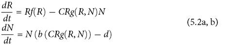
This has the structure of most of the consumer-resource models discussed in pre­vious chapters, except that the functional forms of several components are not specified. The function f describes resource per capita population growth. The con­sumer functional response is a linear response, CR, multiplied by a function, g, which describes the alteration of the linear response form by factors such as handling time, behavioural modification of foraging, and predator (consumer) interference. The increasing function b describes the per capita birth (production) rate as a function of resource intake, and d is a per capita death rate of the consumer. At equilibrium, b = d; this equilibrium condition provides an implicit relationship between d and the value of N at equilibrium.

Abrams (2009c) illustrates how the shapes of the component functions of eqs (5.2) influence the relationship between consumer population size N and consumer per capita mortality rate, d. Some of the main conclusions of that analysis are as follows:

1. Linear forms for f and b, together with a constant value for g (i.e., linear resource density dependence, linear consumer numerical response, and linear consumer functional response) are required to obtain the linear N vs d relationship produced by the logistic model for consumer growth. Empirical studies suggest that this set of three conditions is seldom satisfied.

2. If the only exception to the conditions for a linear N vs d relationship is nonlin­ear resource density dependence, then the consumer ‘inherits’ the same form of density dependence as the resource. Thus, if eq. (5.1) described the resource den­sity dependence in eq. (5.2a), the curvature of the resource per capita growth rate function would also describe the curvature of the consumer’s N vs d relationship. If B is the slope of the numerical response, b, at the equilibrium point then,

Equation 5.3b means that the curvature of density dependence at a particular mortal­ity rate, d, has the same sign as, and is proportional to, the density dependence of the resource at this point. It is important to note that the relationships described by the above two formulas may have major differences from the power law of eq. (5.1). This is true when resource growth, or a large component of it, is based on an abiotic growth model similar to the chemostat model (f = (I/R) - E, with I being input rate, and E being per capita exit rate). This case is treated in Abrams (2009c; Figure 1, p. 324); a model characterized by a linear b, g = 1, and chemostat resource growth produces

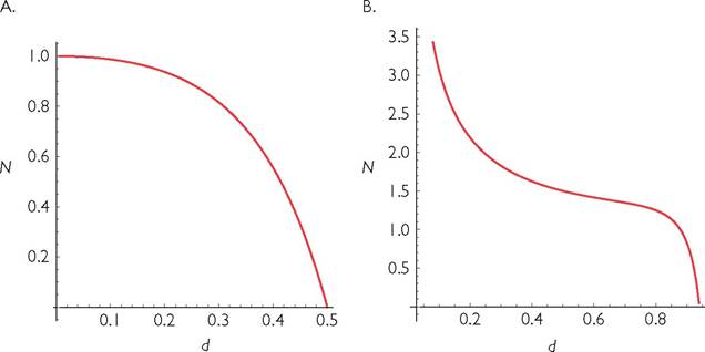
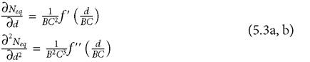
Fig. 5.2 Consumer population size vs mortality for 1-consumer-1-resource systems with a logistic resource and a consumer with a linear numerical response and a type II (panel A) or type III (panel B) functional response. The type II response is a disc equation of the form used for a 2-consumer model in eqs (5.5). The type III response has the same formula except that resource abundance, R is replaced by R². The parameter values in panel A are: B = C = k = r = h = 1. Panel B has identical parameters except that k = 1/4.

a uniformly concave N vs d relationship. However, this is not well approximated by any power-law relationship.

A wide variety of models can exhibit both concave and convex sections in their N vs d relationships. This is true of models with a logistic resource and a type III consumer functional response. It is also true of models that combine abiotic (or par­tially abiotic) growth with a consumer having a type II functional response. These two scenarios are illustrated in Figures 5.2 and 5.3 respectively.

The second major difference between density dependence as represented by eq. (5.1) versus consumer-resource models is that the latter often have a range of mor­tality rates over which the equilibrium consumer abundance rises with increases in its own mortality, i.e., a hydra effect. This was implicit in Rosenzweig and MacArthur’s (1963) analysis of the possibility of cycles in predator-prey systems. They showed that the equilibrium predator abundance increased with predator mortality in unsta­ble systems. However, they did not calculate mean densities in cycling systems, so it was not clear whether mean abundance would actually increase with increas­ing mortality over some range of mortalities. Abrams (2002) showed the potential for an increase in population size with mean density in a system having logistic resource growth and a type II consumer functional response, and Abrams (2009a) examined that relationship for a theta-logistic resource with resource immigration from an external source. The mean and equilibrium abundances can differ greatly, but there are still many cases in which the mean increases with increasing mor­tality (Figure 2 in Abrams 2009a, p. 466). The presence of population cycles makes

Fig. 5.3 Consumer population Sizevsmortalityarisingfrom 1-consumer-1-resource sys­tems with abiotic or partially abiotic resource growth. Panel A describes a system with purely abiotic growth (dR/dt = I - ER), and a consumer with a linear numerical response and a type II functional response (as in eq. 5.4). It has parameters I = E =1; B = C =1; h = 2. Panel B shows consumer population size in a system with summed logistic and abiotic growth components and a type II consumer functional response. It has parameters I = E =0.1; r = k = 1; B = C = 1; h = 5.

any model having the form of eq. (5.1) a poor description of dynamics. Cortez and Abrams (2016) showed that hydra effects can occur in other models for the preda­tor or the prey species in stable predator-prey systems. If the factor causing predator mortality also reduces its capture rate of prey, a much wider range of models and conditions imply an increase in the ultimate population size with an increase in the consumer mortality rate (Abrams 1992b, 2002).

The third qualitatively different outcome of models with explicit resources is the possibility of sustained cycles. These are most often associated with saturat­ing functional responses and self-reproducing resources. However, even within the framework of homogeneous populations with no time delays, cycles are not restricted to biotic resources. Abrams (1989) showed that limit cycle dynamics were possi­ble in a system having an abiotic resource provided the consumer had a functional response that decreased over some range of resource abundances. Such a function­al response was termed ‘type IV' by Holling (1965; also Holling and Buckingham 1976), but most subsequent theoretical articles on functional responses have ignored it. Holling (1965) observed a type IV in experiments at very high prey abundances, and attributed it to disturbance of the predator’s hunting and consumption behaviour being interrupted by the large number of encounters with prey. However, Jeschke et al. (2004) found a number of type IV responses in their review of experimental studies. Abrams (1989) showed that an adaptive functional response should decrease at high levels of foods that contained non-lethal toxins.

The response of the mean consumer population in a cycling population to changes in its mortality rate or other parameters can differ greatly from the corresponding response of the equilibrium point to the same mortality change (Abrams and Roth 1994a, b; Abrams et al. 1998; Abrams 2002, 2009a). The nature of responses of mean densities to consumer mortality in cycling systems has only been examined for a handful of models, mainly 1-consumer-1-resource systems using very simple func­tions for the three basic components. Cycling consumer-resource systems can be characterized by a relationship between the mean consumer abundance and its per capita mortality rate, but those must be determined numerically (as done in Figure

3.2 for a system with two consumers).

The last class of qualitative differences between the potential dynamics of the theta-logistic model (eq. (5.1)) and consumer-resource models is the presence of alternative attractors. Consumer-resource models with relatively simple components can have alternative equilibria or alternative attractors. Bazykin (1974; described in Bazykin 1998) long ago showed that models having a logistic resource and a predator with both a type II functional response and some direct density dependence in its mortality, could have a cyclic and a non-cyclic attractor. Two alternative stable equi­libria are possible in this model. Alternative equilibria also can occur if immigration of the resource is added to a standard model in which the resource is logistic and the predator has a type II functional response (Reynolds and Brassil 2013). In these cas­es, the relationship between population density and mortality can have two (or more) distinct segments (Abrams 2009d, Reynolds and Brassil 2013).

Consumer-resource models should be used in modelling intraspecific competi­tion because of their much wider range of dynamics and frequent inconsistency with single-species density dependence. However, in many cases little or nothing is known about the consumer-resource interaction(s) underlying density dependence. There are also cases in which the resources rapidly reach a quasi-equilibrium state with respect to consumer abundance, without complicated transient dynamics. In either of these circumstances a traditional model of density dependence may be unavoid­able. This leads to the question of what function f should be used in dN/dt = Nf(N)? The most common approach has been to use the per capita growth rate in the logistic or theta-logistic model. If this is done in the future, it would be desirable to at least explore some of the implications of the more common forms of consumer-resource models for the dynamics of the system under consideration.

The consumer-resource models discussed above have largely used the same range of functional components that had been developed in the pre-MacArthur era. That pretty much reflects the range used in the recent models of competition that were reviewed in Chapter 4. Adaptive behaviour is probably the most consequential bio­logical process omitted from these models. The need to consider adaptive behaviour in models of consumer-resource interactions was first suggested by William Mur­doch in his work on switching behaviour in predators (Murdoch 1969). Incorpo­rating foraging behaviour into models now encompasses a reasonably large body of literature. However, adaptive food choice has been more influential in behavioural ecology than in population or community ecology.

I incorporated the types of behaviourally influenced functional responses dis­cussed in Chapter 3 into food chain models in a series of articles beginning in 1984 (including Abrams 1984b, 1990c, 1992c, 1995). Some of these treated 3- and 4-level systems. They all suggested that adaptive balancing of food intake rate and predation risk could produce very different models for the growth of the top species in a food chain than were present in typical 2-level consumer-resource systems. For example, Abrams (1995) examined a simple 3-level food chain model with linear functional responses, logistic growth of the basal resource, and nonlinear numerical responses for both consumer species. It had the potential for adaptive behavioural balancing of food intake and predation risk by the mid-level species. This allowed the abun­dance of the bottom-level species to have the same (negative) immediate effect on the per capita growth rate of the top species as did the abundance of that top-level species (eqs (9) in Abrams (1995)). Neither of these immediate effects existed in the model without behavioural flexibility of the mid-level species. The mid-level species' behaviour also allowed for a hydra effect in the top-level species. Increased abundance of the bottom-level species reduced its rate of mortality due to its consumer. All these behaviourally generated changes in the per capita growth rate are incompatible with simple models of density dependence having a form similar to eq. (5.1).

Since the development of basic theory about anti-predator behaviour in food chains in the 1990s, considerable empirical evidence for the type of adaptive forag­ing envisioned in those models has accumulated (Werner and Peacor 2003; Bolnick and Preisser 2005). However, the nature of the impact of these behaviours on the relationship between mortality and population productivity of a top-level consumer species has received relatively little attention since my 1995 article discussed above. Abrams (2009d) showed that adaptive defence was another possible mechanism that could produce changes in the curvature of the relationship between consumer per capita mortality and consumer population size, as well as alternative attractors (Fig­ure 4 of Abrams 2009d, p. 300). Abrams and Vos (2003) had earlier demonstrated that several counter-intuitive responses of species to mortality (either their own or one of the other species) occurred in a food chain where each level could have direct negative intraspecific effects on immediate growth rate, and the middle level var­ied its traits adaptively to balance increased food intake with its associated increased predation risk.

5.2.4 One-consumer-multi-resource systems

As noted above, specialist consumer-resource systems are rare. However, the possi­bility of systematic differences in the shape of density dependence between specialist and generalist consumers has received very little attention, as noted in Abrams (2009b). Having two or more resources implies the existence of indirect interac­tion^) between those resources, transmitted via the consumer (due to consumer satiation and effects on consumer abundance). In addition, there are often other interactions between the resources, including competition for their own foods when they are biotic. Finally, active resource choice by the consumer can greatly alter the indirect component of interaction between resources that is transmitted via the consumer.

This section will use the approach of the previous one in exploring the shape of the relationship between equilibrium or average population size and a constant addi­tional per capita mortality. This is the best description of the effect of intraspecific competition in systems where resource dynamics imply that a single-species density dependent growth model cannot adequately describe the process of self-limitation. Many of the qualitatively different behaviours of models with multiple resources are exhibited by the simplest case, in which there are just two resources, so that is the only case considered here. Biotic and abiotic resources are considered, as are situations with and without interactions between the resources.

Having a consumer with two resources that do not interact directly differs from single-resource systems when the two resources differ from each other, either in their growth functions or their susceptibility or value to the consumer. A potential choice of resources means that there are a variety of adaptive behaviours that may affect the form of the consumer’s functional responses. The consumer maybe able to increase consumption of one resource at the expense of decreased consumption of the other. When the resources are nutritionally substitutable, this involves increased relative consumption of the resource that can be caught more rapidly, meaning that the attack rate parameter C_i increases with R_i (Abrams 1987c, Abrams and Matsu­da 2004). When resources are nutritionally essential, a decrease in the attack rate, C, on the more abundant resource is likely, as the less abundant one is then likely to be more limiting (Abrams 1987c). If the original relationship between mortality and abundance is linear, choice will generally make it nonlinear. In addition to affecting consumer choice, the abundance of the second resource may change the optimal level of general foraging effort, producing other indirect interactions between the different resources.

I will first consider a system with two resources in which the consumer is unable to alter its ‘attack rates’, C_i, on the resources. If the two resources differ in their sus­ceptibility (C) to the consumer, the N vs d relationship is changed from that in a comparable single-resource system. Given a difference in C-values, a smaller con­sumer death rate increases the relative contribution of the lower-C resource to the consumer’s diet. A sufficiently low death rate results in exclusion of the more vulner­able resource when the consumer does not exhibit any adaptive switching behaviour. Figure 5.4 provides an example of a system in which the consumer is characterized by a multi-species type II response (see Box 2.1) and the two resources have logistic growth (dR/dt = m + R(r - kR), where m is a very low rate of immigration). The sys­tem exhibits cycles over abroad range of consumer death rates. Resource 1 is captured at 1/5 the rate of resource 2, which means resource 2 is susceptible to extinction. The three panels show cases with different r-values for resource 1. All the panels show the equilibrium consumer population size as a function of its per capita mortality rate. A low enough consumer death rate causes extinction of the more vulnerable resource, and stable dynamics. As the death rate is raised, the second resource returns, which in turn causes a relatively abrupt change in system dynamics to cycles. The dynamics

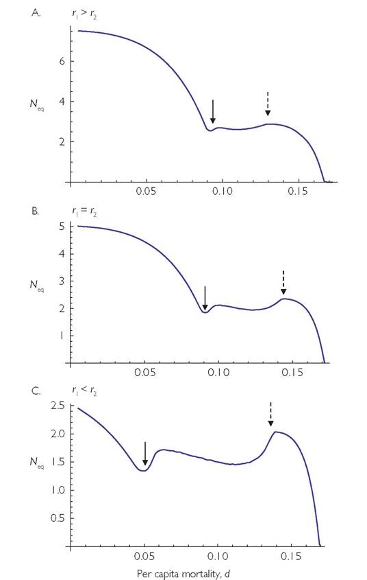
Fig. 5.4 Equilibrium consumer population size as a function of consumer per capita mor­tality rate, for systems with two logistic resources. 'The dynamics assume external resource immigration at a rate m for both resources. The parameters that are common to all panels are: B = 1; m = 0.0001; k = 1; Ci = 0.2; C₂ = 1; h = 5; r₂ = 1. In panel A, r₁ = 1.5, in panel B, r₁ = 1 (= r₂), and in panel C, r₁ = 0.5. The solid arrows give the point at which the more vul­nerable resource (resource 2) is able to achieve a significant density (i.e., where it would persist without immigration), and the dashed arrows denote the mortality rate above which the system with both resources becomes stable.

switch again from cyclic to stable at sufficiently high consumer mortality rates. The overall shape of the N vs d relationship in all three panels is one with convex sections at low and high mortalities, separated by a relatively flat intermediate section over which there are population cycles. In this section, the mean consumer density is only slightly higher than the equilibrium shown here.

Abrams (2009b) illustrated the form of N vs d for a system with very many resources types that are characterized by a continuous range of different C-values. As consumer mortality is increased from very low values, extinct or nearly extinct resources can return to the system, resulting in a continuous increase in mean resource vulnerability, and a concave N vs d at low mortality rates, d. At high con­sumer mortality, all resources are present, and the consumer’s type II functional response then leads to a convex relationship with a sharp and accelerating decline in equilibrium consumer abundance to zero as mortality approaches its maximum value. As Holt (1977) demonstrated, the most extinction-prone resources are gen­erally those characterized by the greatest ratios of the consumer’s attack rate to the resource’s maximum per capita growth rate in the absence of the consumer. The loss of a resource species due to this apparent competitive exclusion produces a decrease in mean resource vulnerability to consumption and/or a decrease in total resource productivity as the death rate of the consumer is decreased. When combined with the fact that functional responses must saturate at a high enough resource abundance (high enough predator mortality), this also suggests that the most likely relation­ship between per capita mortality rate and population size is one that is concave (decelerating) at low mortality and convex (accelerating) at high mortality.

The models considered thus far lack adaptive foraging by consumers or defensive behaviour by resources. If the two resource types are caught using different foraging behaviours, or are found in different locations, the consumer can usually adapt quick­ly to increase its capture rate of the currently more rewarding resource. This usually entails a reduction in its capture of the less rewarding resource. The impacts of such dynamic switching behaviours were examined in Abrams and Matsuda (2003, 2004). McCann et al. (1998) and McCann (2012) represented switching using a response that is a special case of Abrams and Matsuda (2003). Subsequent works with more complex procedures for representing switching functional responses were later pro­posed by van Leeuwen et al. (2013) and Morosov and Petrovskii (2013). Allvarieties of switching responses tend to equalize the intake rates of alternative resources. As a result, extinction of one resource following a lowering of the consumer death rate occurs over a smaller range of mortality rates, or may not occur at all. However, the possibilities of unstable equilibria and of different potential forms for the dynamics of behavioural change again introduce complications. The impact of switching on the relationship between mortality and consumer population size does not appear to have been studied. Figure 5.5 presents an example using the very simple switching func­tion that was used by Abrams and Matsuda (2003). With two or more prey (resource) types, switching multiplies the attack rate on resource i, Ci, by the function:

(C_lR_l )^z

(5.4)

∑ (CjRjY

j=1

where ω is the number of resource types, and z is an exponent that roughly affects the accuracy of the behavioural switching. (Larger values of z imply a greater ‘preference’ for the most abundant resource(s); see Abrams and Matsuda (2003).) With z = 0 the intake rates of all the resources are proportional to their attack rates, so there is no adaptive preference. Figure 5.5 shows the impact of incorporating switching on the mortality vs population size relationship in a 1-consumer-2-resource system. Each of the two panels compares systems with and without switching; panel A assumes linear functional responses, while panel B assumes type II responses. Switching prevents the extinction of the more rapidly caught prey that can occur at low predator mortality rates. Switching also expands the upper limit of the mortality rates allowing consumer existence. Switching maintains the generally concave shape of the relationship pro­duced by models with linear functional responses and non-interacting resources, but alters the details of the shape. Although it is not shown in the figure, switching also changes the range of parameters that allows population cycles. In addition, switching significantly alters the nature of those cycles. Either switching or cycles alone would likely change any quantitative measure of the interaction.

In the models discussed above, the only linkage between the population dynamics of different resources has been via their shared consumer. There is also the possibility that resources (prey) compete for lower-level resources. The impact of competition between resources is illustrated by the simplest model of the ‘diamond food web’ (Leibold 1996; Noonburg and Abrams 2005), which embodies this food web struc­ture. The diamond web involves a single basal resource (with population R), con­sumed by two mid-level prey species (N ₁ and N₂), which are in turn consumed by a single predator (P). Coexistence of the prey in a stable system requires that the one that is better at resource exploitation (has a lower R* in the absence of the predator) must be more susceptible to the predator. Without the predator, one prey (the one with the lower R*) would exclude the other. If a low level of external immigration is added for both prey, the otherwise-excluded prey persists at a very low abundance.

The simplest (and most common) model of the diamond web assumes linear func­tional responses of all consumer species and logistic growth of the basal resource. If both prey species are present, mortality applied to the predator has no effect on its equilibrium abundance. An increase in the predator’s mortality brings about a short­term decrease in its abundance, but the resulting increase in the relative abundance of the more vulnerable prey restores the predator’s original abundance. If the predator were maintained at any fixed abundance, one of the two prey would be excluded, as this would imply two competing prey with a single limiting factor (the shared resource). There is no effect of an increased per capita mortality rate on the predator’s population size. Of course, a sufficient change in the mortality rate of the predator will cause extinction of one of the prey; the predator-resistant prey will go extinct at high enough predator mortality rates, and the superior resource exploiter will go extinct at

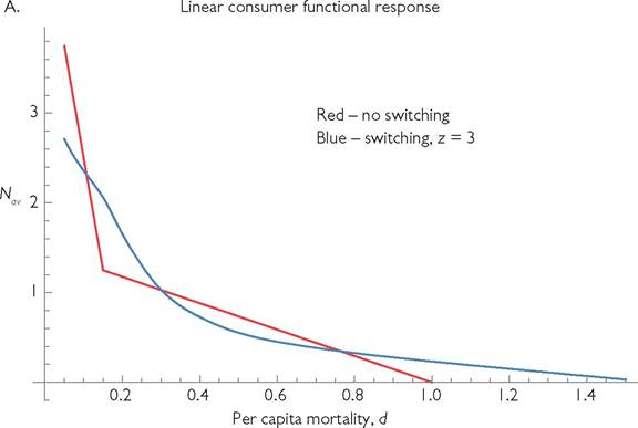
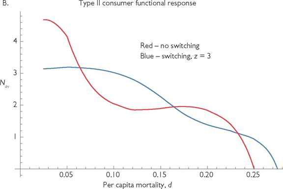
Fig. 5.5 'The effect of mortality on the population size of the consumer in a system with two logistically growing resources and a single consumer species that may exhibit switching behaviour. In panel A, the consumer has a linear functional response, and in panel B, it has a type II functional response with a handling time, h = 3. In each panel, the red line represents the mean population vs mortality (d) relationship in the absence of switching, the blue line is a switching predator characterized by the exponent z = 3 in eq. (5.4). The other parameters are; ω = 2; r_i = 1; k_i = 1, Ci = 0.8, C₂ = 0.2; B_i = 1.

predator mortality rates below a lower threshold value. In either case, the slopes of the relationships between per capita mortality and predator population size and between per capita mortality and predator production (predator population growth rate) will change abruptly when the extinction occurs. The web and the resulting relationships between predator mortality and predator population size are shown in Figure 5.6A, while the resulting relationship between the productivity of the predator population and mortality is shown in Figure 5.6B. The latter has a minimum close to one-half of the mortality that would cause the top predator extinction. This contrasts sharply with the prediction arising from a logistic model of the predator’s growth, in which mortal­ity that was half of the maximum allowing existence would maximize the productivity of the population.

Giving the predator a type II (disc equation) functional response changes the dynamics of the diamond food web considerably. Here I assume a multi-species disc equation with equal nutritional values and handling times for the two prey species (Abrams and Matsuda 2005). In this case, increasing predator mortality often increas­es its abundance; i.e., higher average predator abundances are associated with larger (rather than smaller) per capita growth. Abrams and Matsuda (2005) proposed the general term ‘hydra effect’ to apply to this and any other scenario in which greater mortality of a given species led to a greater equilibrium population size. As was not­ed above, the hydra effect also occurs in the simple 2-species model with a type II predator and a logistically growing prey. Here, it has been known since 1963 (Rosen- zweig and MacArthur 1963) that increasing predator mortality in an unstable system will increase the equilibrium predator abundance (see e.g., Abrams 2002,2009a). The basic mechanism is that greater predator mortality increases the prey abundance, which leads to a larger amount of‘handling’. If the predator is initially overexploiting the prey (prey abundance less than the level that maximizes the population rate of increase), a lower effective capture rate (due to the increased total handling time) can increase the predator’s abundance. This is somewhat complicated by the fact that mean abundance in cycling systems in this model can be much greater than the equilibrium abundance. However, this does not change the fact that mean predator abundance goes up with increases in its own mortality over some range of mortalities. When the system is at equilibrium, the imposed per capita mortality is again equal to the predator’s per capita production rate, so higher mortalities are again associated with greater population production, contrary to standard density dependence.

Another scenario involving shared predation occurs when two prey species con­sume different biotic resources, and each prey adaptively adjusts its foraging time or rate based on the commonly observed trade-off between food intake and predation risk (Lima and Dill 1990). Abrams (1984b) analysed the single-prey version of this scenario, and Abrams (1987d) extended it to a predator with two prey, each with its own resource. In the two-prey system, adaptive prey behaviour can lead to an increase in the first prey’s equilibrium density after adding the second prey. The basic mechanism is that the increase in the predator abundance after adding the second prey causes the first prey to exploit its resource at a lower rate, causing an increase in resource abundance that more than compensates for the lower capture rate.

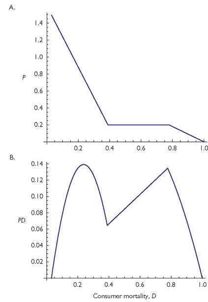
Fig. 5.6 Panel A illustrates the effect of the per capita mortality rate of the top consumer on its population density for the simplest diamond food web with linear functional components. This model has the form:

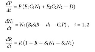
The minimum per capita mortality (D) of the predator is assumed to be 0.03; all additional mortality is assumed to be due to harvesting. Panel B shows the corresponding relationship between total death rate of the predator and amount harvested in this same food web. The parameter values are: C₁ = 0.25; C₂ = 1; S₁ = 0.5; S₂ = 1; d₁ = d₂ = 0.1; E₁ = E₂ = 1.

5.2.5 A more mechanistic approach to density dependence

Models of purely density-dependent growth continue to be common in the literature. Theoreticians use density-based models of growth to simplify multi-species models, which makes them easier to analyse. They are particularly likely to be used for species at the bottom trophic level of the food web when the focus of interest is a higher trophic level. I have certainly been guilty of this in many articles. Fisheries biolo­gists (and others dealing with resource management) still frequently use models of single-species density-dependent growth for species at higher trophic levels. This is presumably because the relationships of population growth to resources and other factors are largely unknown for the species in question. Textbooks give detailed cover­age to density-based models. This is perhaps due to historical inertia or the simplicity (and consequent pedagogical utility for a mathematically unsophisticated audience) of the models. All models require some simplifications, but it is vital to be aware of the phenomena and outcomes that may be rendered invisible by such simplifica­tions. Loreau (2010, and elsewhere) has argued for including all lower trophic levels explicitly in models of population growth, and this approach should be used to veri­fy whether assumptions of logistic resource growth affect the qualitative results of a model of competition.

The common view that consumer population density is the sole or main deter­minant of its per capita population growth rate has no doubt inhibited experimental approaches that could provide a better understanding of single-consumer popula­tion growth. The response of consumer population growth to a change in its own abundance is always affected by resources, which seldom, if ever, reach a new equilib­rium instantaneously when the number of consumer individuals changes. Chapters 8 and 9 will illustrate some of the consequences of these delays in seasonally varying environments.

5.3