Predator-prey cycles can be modeled mathematically

One way to evaluate possible causes of population cycles is to investigate the issue mathematically. In the 1920s, Alfred Lotka and Vito Volterra independently represented the dynamics of predator-prey interactions with what is now called the Lotka-Volterra predator-prey model:

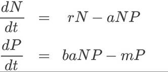
(12.1)

In these equations, N represents the number of prey individuals and P represents the number of predator individuals.

Predators starve when there are no prey. Thus, the equation for change in the predator population over time (dP/dt) assumes that in the absence of prey (N = 0), the number of predators decreases exponentially with a mortality rate of m

(i.e., dP/dt = -mP). When prey are present (N ≠ 0), individuals are added to the predator population according to the number of prey that are killed (aNP) and the efficiency with which prey are converted into predator offspring (represented by the constant b). Thus, the rate at which individuals are added to the predator population is baNP.

We can determine the relationship between prey and predator populations by solving for the population growth equation of each species (Equation 12.1) when they stop changing in size (or reach an equilibrium). This approach involves determining the zero population growth isocline for both prey and predator. The zero population growth isocline (or simply isocline) is the condition in which the population size of the prey (or the predator) does not change in size for a given number of predators (or prey). For prey, their abundance does not change when dN/dt = 0, which occurs when P = r/a. Similarly, the abundance of predators does not change when dP/dt = 0, which occurs when N = m/ba.

Once we determine r/a and m/ba, we can then plot the isocline for both the prey (x-axis) and predators (ó-axis) in graphical form. For the prey, the isocline will be a horizontal line originating at the value P = r/a (FIGURE 12.14A). This line represents the number of predators needed to keep the prey population from changing (or at equilibrium). If the predator abundance is below the line, the prey population will increase in size. If the predator abundance is above this line, then the prey population will decrease in size. Similarly, for the predator, the isocline will be a vertical line originating at the value N = m/ba (FIGURE 12.14B). This line represents the number of prey needed to maintain the predator population at zero growth. If the prey abundance is to the left of the line, the predator population will decrease in size. If the prey abundance is to the right of the line, then the predator population will increase in size.

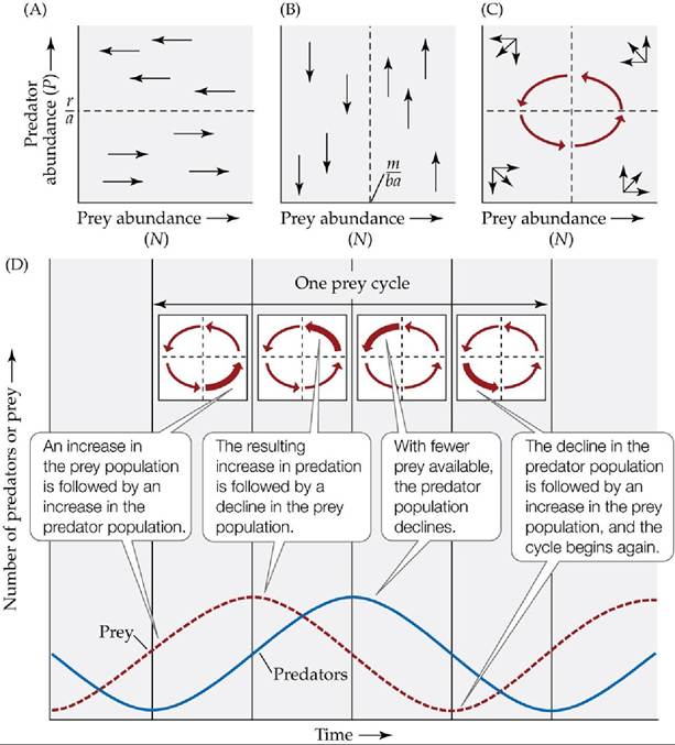
FIGURE 12.14 The Lotka-Volterra Predator-Prey Model Produces Population Cycles

(A) Considering the prey population first, the abundance of prey does not change when dN/dt = 0, which occurs when P = r/a (see Equation 12.1). (B) Similarly, considering the predator population, the abundance of predators does not change when dP/dt = 0, which occurs when N = m/ba.

Combining the isoclines in Figure 12.14A,B shows that the isoclines cross at 90° angles and divide the graph into four regions (FIGURE 12.14C). We can then follow the population growth of both predator and prey in each of these regions and find that both cycle over time, with the predators lagging behind the prey by one-fourth of a cycle (FIGURE 12.14D). Starting in the lower right corner, both prey and predator populations are growing but the increasing numbers of predators cause the prey abundance to level off and eventually reach zero population growth at its isocline. As the populations move into the upper right corner, predator abundance is still increasing but prey abundance is in decline. This causes the predator population to slow its growth and eventually reach its isocline. Now the prey population has declined to the point that the predator population cannot sustain itself and it declines as well (upper left corner). Finally, in the lower left corner, the prey population rebounds because of low predator numbers and begins to increase. This increase eventually leads to an increase in predators when the cycle starts all over again.

The Lotka-Volterra predator-prey model thus yields an important result: it suggests that predator and prey populations have an inherent tendency to cycle because the abundance of one population is dependent on the abundance of the other population.

Predator-prey cycles can be reproduced under laboratory conditions

Can the cycling behavior of predator-prey models be reproduced in the laboratory? Experiments show that such cycles can be difficult to achieve. When prey are easy for predators to find, predators typically drive prey to extinction, then go extinct themselves. Such was the case in C. B. Huffaker's experiments with the herbivorous six-spotted mite (Eotetranychus sexmaculatus) and the predatory mite, Typhlodromus occidentalis, that eats it (Huffaker 1958). In an initial set of experiments, Huffaker released 20 six-spotted mites on a tray with 40 positions, a few of which contained oranges, which these herbivorous mites could eat (FIGURE 12.15A). At first, the six-spotted mite population increased, in some cases reaching densities of 500 mites per orange. Eleven days after the start of the experiment, Huffaker released two predatory mites on the tray. Both prey and predator populations increased for a time, then declined to extinction (FIGURE 12.15B).

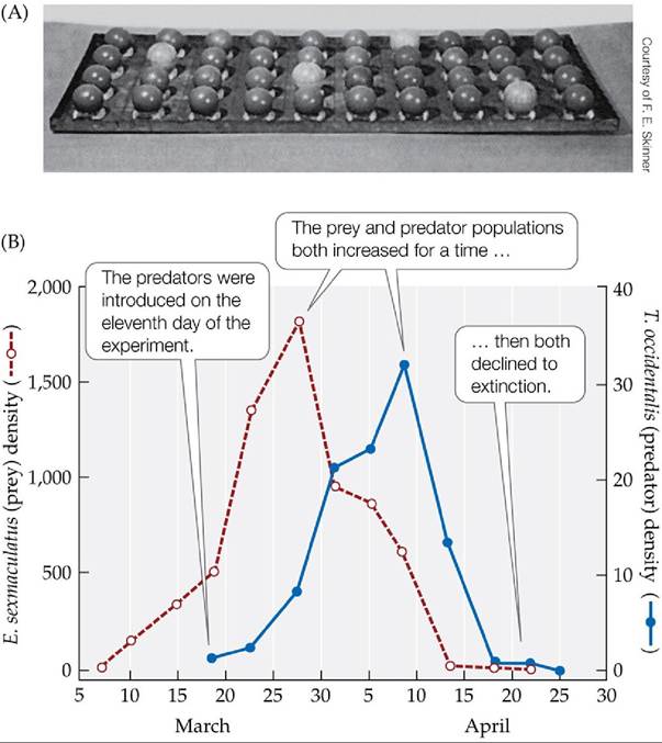
FIGURE 12.15 In a Simple Environment, Predators Drive Prey to Extinction (A) C. B.

Huffaker constructed a simple laboratory environment to test for conditions under which predators and prey would coexist and produce population cycles.

Huffaker observed that the prey persisted longer if the oranges were widely spaced—presumably because it took the predators more time to find their prey. He tested this idea in a follow-up experiment in which he increased the complexity of the habitat in the following way. First, he added strips of Vaseline that partially blocked the predatory mites as they crawled from one orange to another. Then he placed small wooden posts in an upright position on some of the oranges; these posts allowed the six-spotted mites to take advantage of their ability to spin a silken thread and float on air currents over the Vaseline barriers. Thus, he altered the experimental environment to favor dispersal of the six- spotted mite and impede dispersal of the predatory mite. Under these conditions, the prey and the predators both persisted, illustrating a form of “hide-and-seek” dynamics that produced population cycles (FIGURE 12.16). The six-spotted mites dispersed to unoccupied oranges, where their numbers increased. Once the predators found an orange with six-spotted mites, they ate them all, causing both prey and predator numbers on that orange to plummet. In the meantime, however, some six-spotted mites dispersed to other portions of the experimental environment, where they increased in number until they too were discovered by the predators.

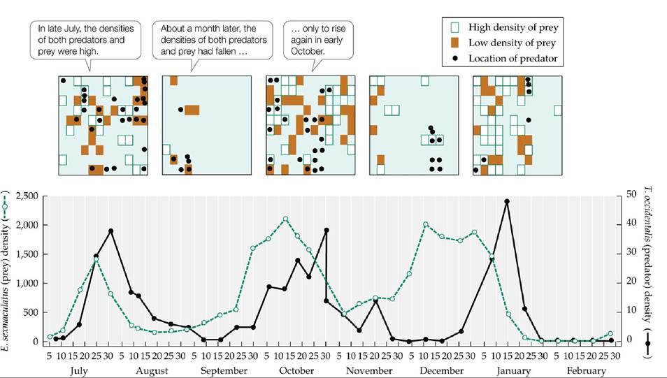
FIGURE 12.16 Predator-Prey Cycles in a Complex Environment Huffakermodifiedthe simple laboratory environment shown in Figure 12.15 to create a more complex environment that aided the dispersal of the prey species but hindered the dispersal of the predator. Under these conditions, predator and prey populations coexisted, and their abundances cycled over time. The top panels show the locations within the environment of prey (shaded regions) and predators (circles) at five different points in time. (After C. B. Huffaker. 1958. Hilgardia 2T: 343-383.) View larger image