The Lotka-Volterra model

Because this book will be mainly about theory, it is necessary to begin with a brief review of the foundational mathematical model of interspecific competition, even though that model lacks any representation of resources.

The Lotka-Volterra (LV) model notably lacks any explicit representation of resources. It assumes that the per individual rate of increase of each consumer (com­petitor) species declines linearly with increases in its own abundance and declines linearly (usually with a different slope) with increases in the abundances of the second consumer species. The effects of changes in abundance on per individual growth rates are immediate. The most common representation of the LV model of two-species competition describes the rates of change in their abundances (N₁, N₂) as follows:

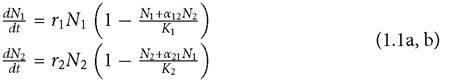
The parameters r_i and K_i are respectively the maximum per individual growth rate and the equilibrium population size (‘carrying capacity') of species i when it is present alone. The effect of interspecific relative to intraspecific competition is measured by α_ij, which is the ratio of the effect of the abundance of species j on the per capita rate of increase of species i, relative to the effect of the abundance of species i on its own per capita growth rate. The competition coefficient α_ij increases with the similarity of the two species in their relative use of different resources; it also increases as the absolute ability of species j to harvest all resources increases relative to that of species i.

One outcome that was not widely appreciated before the development of the LV model was that in some cases when interspecific competition is stronger than intraspecific (α₁₂α₂₁ > 1), either species is capable of excluding the other, with the outcome depending on initial abundances. In the two-species LV model, it is possi­ble to determine whether the species will coexist by examining the growth rate of each species when it is very rare and the other species is at its carrying capacity. Ifboth of these ‘invasion growth rates' are positive, the two species will coexist, and if not, coex­istence is impossible. Both invasion growth rates are negative in the case of alternative outcomes. Alternative outcomes were observed in later laboratory experiments.

The sets of outcomes in the LV model are usually illustrated using ‘isocline dia­grams’.

Unfortunately, the conditions for coexistence in the two-species LV model do not apply universally to models that have explicit resource dynamics, or to models with temporal variability, or to a range of other models and the consumer-resource interactions that underlie them. There is no analogue to the two-species coexistence condition LV model with three or more competitors. In any LV model, each species’ population growth rate responds immediately to a change in the other species, something that is usually not the case for real consumer-resource interactions. Even when the LV model is being used as a rough approximation, estimating the parame­ters of the model from first principles—particularly the strength of competition given by the α values—requires a consumer-resource model. These and many other limi­tations of models lacking explicit resource dynamics will be discussed in this book. However, it should be noted that Volterra did include resources in his conceptualiza­tion of competition, even though he did not use the term. This is evident in his idea that only a single species could persist indefinitely if there was only a single limiting factor, or, as it later came to be known, the ‘competitive exclusion principle’.

The limitation to a single consumer on a single resource follows from the two- species competition model when the product of the competition coefficients is equal to or greater than one. If there is purely exploitative competition for a single resource by two consumers, the product of their competition coefficients is unity, and there will be either no equilibrium point with positive densities of both, or, for a unique ratio of carrying capacities, a line of neutrally stable points. Volterra pointed out that the species that persist at the lowest level of that factor would prevent the existence of (i.e., exclude) all the others. Hardin (1960) notes that some authors later attributed this idea to Gause (1936), who had carried out a laboratory experiment in which competitive exclusion occurred. Hardin also noted that a wide range of authors had proposed similar ideas before and after Volterra. Many more recent authors attribute the idea to Tilman (1982).

In any case, the issue of coexistence on a single resource has remained a topic of continued interest, largely because early authors did not devote much thought to what exactly constitutes a single resource. Haigh and Maynard Smith (1972) suggest­ed that the same resource species (or substance) at different times could constitute different resources, as could different parts of an individual of the resource species. Stewart and Levin (1973) and Armstrong and McGehee (1976a, b) showed that the prohibition of coexistence on a single resource type did not apply to consumer species in seasonal environments or species undergoing sustained population cycles. There has now been a large body of work (summarized in Chesson 2020b) on the potential for environmental variation to allow coexistence on a single resource. However, this requires that the consumers differ in their temporal responses to changing resource densities, in which case resource items becoming available at different times could be divided into different classes of resources.

In spite of its limitations, the LV model did reveal some properties of at least some two-competitor systems, which were not widely appreciated in the 1920s. In addition, Lotka and Volterra’s works inspired some early experimental explorations of competi­tion in the laboratory by Georgy Gause (1936), who studied competition between two protozoans, and by Thomas Park (1948), who did the same for a pair of flour beetle species. These were the first influential experimental approaches to understanding competition in biological communities. Each of these authors related their results to the LV model. However, they were mainly concerned with examining whether or not competitive exclusion occurred in pairs of species, and did not really provide a challenging test for the adequacy of the model.

While the LV model played a key role in the birth of competition theory, it was clearly too simple to understand the composition of natural communities, or predict changes in those communities. Its assumption of linear effects on abundance, its focus on only two competing species, and the absence of an explicit accounting of resources combine to greatly restrict the ability of the LV model to describe any natural sys­tem, or even the majority of laboratory systems. This became clear many years later, after Francisco Ayala (1969) published a study on competition between Drosophila species in the laboratory in the journal Nature. His assumption that the LV mod­el applied exactly to his two-species competition experiments led him to conclude that his observation of coexistence invalidated the competitive exclusion principle.

Ecology is certainly not alone in attempting to understand very complex systems in which it would be unrealistic to develop a quantitative understanding of all of the dynamic components that could influence changes in variables of interest. The normal course of theoretical development of a scientific field would have seen an exploration of the consequences of the most basic elaboration of the model; in this case that elaboration is clearly to include the dynamics of the resources that are the subject of the competitive interaction. This second stage of development was initiated in the late 1960s and early 1970s, but it seems to have been largely abandoned before it was given a chance to restructure the field.

1.4