ACCOUNTING FOR THE EVIDENCE: MODELS AND PREDICTIONS

15.5.1 Shocks Versus Steady States

How can we account for the historical evidence on the evolution of the aggregate wealth-income ratio, the concentration of wealth, and the share of inherited wealth? In this section, we describe the theoretical models that have been developed to address this question.

We are primarily concerned here about the determinants of long-run steady states. In practice, as should be clear from the historical series presented above, real-world econ­omies often face major shocks and changes in fundamental parameters, so that we observe large deviations from steady states. In particular, the large decline in the aggregate wealth­income ratios β_t between 1910 and 1950 is due to the shocks induced by the two World Wars. By using detailed series on saving flows and war destructions, one can estimate the relative importance of the various factors at play (Piketty and Zucman, 2014). In the case of France and Germany, three factors of comparable magnitude each account for approx­imately one-third of the total 1910-1950 fall of β_t: insufficient national savings (a large part of private saving was absorbed by public deficits); war destructions; and the fall of relative assets prices (real estate and equity prices were historically low in 1950-1960, partly due to policies such as rent control and nationalization). In the case of Britain, war destructions were relatively minor, and the other two factors each account for about half of the fall in the ratio of wealth to income (war-induced public deficits were partic­ularly large).^[44]

In thinking about the future, is the concept of a steady state a relevant point of ref­erence? Historical evidence suggests that it is.

We show that over a wide range of models, the long-run magnitude and concentra­tion of wealth and inheritance are a decreasing function ofg and an increasing function of r, where g is the economy’s growth rate and r is the net-of-tax rate of return to wealth. That is, under plausible assumptions, both the wealth-income ratio and the concentra­tion of wealth tend to take higher steady-state values when the long-run growth rate is lower and when the net-of-tax rate of return is higher. In particular, a higher r — g tends to magnify steady-state wealth inequalities. Although there does not exist yet any rigorous calibrations of these theoretical models, we argue that these predictions are broadly consistent with both the time-series and cross-country evidence. These findings also suggest that the current trends toward rising wealth-income ratios and wealth inequality might continue during the twenty-first century, both because of population and productivity-growth slowdown, and because of rising international competition to attract capital.

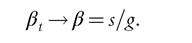
15.5.2 The Steady-State Wealth-Income Ratio: β = s/g

The most useful steady-state formula to analyze the long-run evolution of wealth­income and capital-output ratios is the Harrod-Domar-Solow steady-state formula:

With s = long-run (net-of-depreciation) saving rate, g = long-run growth rate.^[46]

The steady-state formula β = s/g is a pure accounting equation.

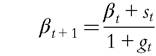
With 1 + g_t = Y_t+1∕Y_t = growth rate of national income, s_t = S_t∕Y_t = net saving rate.

It follows immediately that if s_t → s and g_t →g, then β_t → β = s/g.

The Harrod-Domar-Solow says something trivial but important in a low-growth economy, the sum of capital accumulated in the past can become very large, as long as the saving rate remains sizable.

For instance, if the long-run saving rate is s = 10%, and if the economy permanently grows at rate g = 2%, then in the long run the wealth-income ratio has to be equal to β = 500%, because it is the only ratio such that wealth rises at the same rate as income: s∕β = 2% = g. If the long-run growth rate declines to g = 1%, and the economy keeps sav­ing at rate s = 10%, then the long-run wealth-income ratio will be equal to β = 1000%.

In the long run, output growth g is the sum of productivity and population growth. In the standard one-good growth model, output is given by Y_t = F(K_t, L_t), where K_t is non­human capital input and L_t is human labor input (i.e., efficient labor supply). L_t can be written as the product of raw-labor supply N_t and labor productivity parameter h_t. That is, L_t = N_t ■ h_t, with N_t = N₀ ■ (1 + n)^t (n is the population growth rate) and h_t = h₀ ∙ (1 + h)^t (h is the productivity growth rate).

The long-run saving rate s also depends on many forces: s captures the strength of the various psychological and economic motives for saving and wealth accumulation (dynas­tic, life cycle, precautionary, prestige, taste for bequests, etc.). The motives and tastes for saving vary a lot across individuals and potentially across countries. Whether savings come primarily from a life cycle or a bequest motive, the β = s/g formula will hold in steady state. In case saving is exogenous (as in the Solow model), the long-run wealth-income ratio will obviously be a decreasing function of the income growth rate g. This conclusion, however, is also true in a broad class of micro-founded, general equi­librium models of capital accumulation in which s can be endogenous and can depend on g. That is the case, in particular, in the infinite-horizon, dynastic model (in which s is determined by the rate of time preference and the concavity of the utility function), in “bequest-in-the-utility-function” models (in which the long-run saving rate s is deter­mined by the strength of the bequest or wealth taste), and in most endogenous growth models (see box below). In all cases, for given preference parameters, the long-runβ = s/g tends to be higher when the growth rate is lower. A growth slowdown—coming from a decrease in population or productivity growth—tends to lead to higher capital-output and wealth-income ratios.

Box: The steady-state wealth-income ratio in macro models

Dynastic Model

Assume that output is given by Y_t = F(K_t, L_t), where K_t is the capital stock and L_t is efficient labor and grows exogenously at rate g.

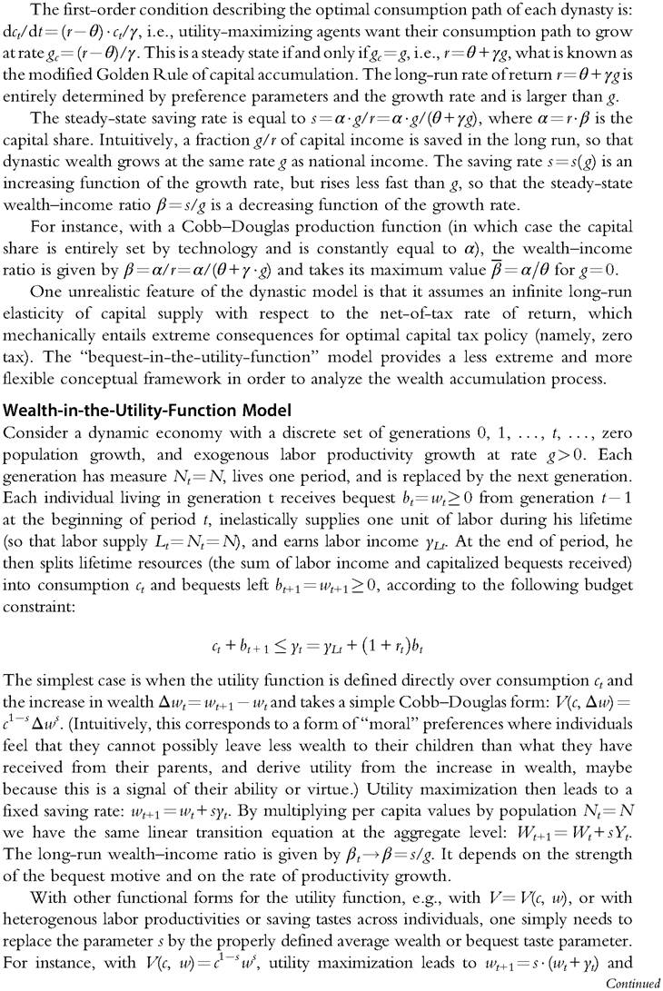
The slowdown of income growth is the central force explaining the rise of wealth­income ratios in rich countries over the 1970-2010 period, particularly in Europe and Japan, where population growth has slowed markedly (and where saving rates are still high relative to the United States). As Piketty and Zucman (2014) show, the cumulation of saving flows explains the 1970-2010 evolution of β in the main rich countries rela­tively well. An additional explanatory factor over this time period is the gradual recovery of relative asset prices. In the very long run, however, relative asset-price movements tend to compensate each other, and the one-good capital accumulation model seems to do a good job at explaining the evolution of wealth-income ratios.

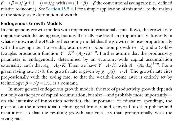
It is worth stressing that the β = s/g formula works both in closed-economy and open­economy settings. The only difference is that wealth-income and capital-output ratios are the same in closed-economy settings but can differ in open-economy environments.

In the closed-economy case, private wealth is equal to domestic capital: W_t = K_t.^[47] National income Y_t is equal to domestic output Y_dt = F(K_t, L_t). Saving is equal to domes­tic investment, and the private wealth-national income ratio β_t = W_t∕Y_t is the same as the domestic capital-output ratio β_kt = K_t∕Y_dt.

In the open economy case, countries with higher saving rates s_a > s_b accumulate higher wealth ratios β_a = s_a∕g > β_b = s_b∕g and invest some their wealth in countries with

33

Figure 15.24 World wealth/national income ratio, 1870-2100.

saving rate at about 12%. Under these (arguably specific and uncertain) assumptions, the world β would rise to about 700-800% by the end of the twenty-first century.

O'—1

15.5.3 The Steady-State Capital Share: α=r∙β=a∙β s

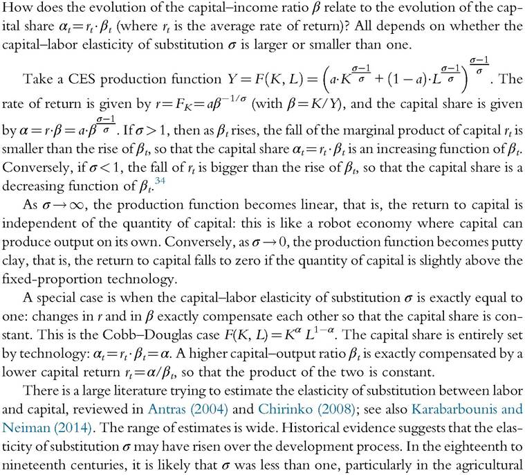
sector. An elasticity less than one would explain why countries with large quantities of land (e.g., the United States) had lower aggregate land values than countries with little land (the Old World). Indeed, when σ < 1, price effects dominate volume effects: when land is very abundant, the price of land is extremely low, and the product of the two is small. An elasticity less than 1 is exactly what one would accept in an economy in which

^[1] Because we include all forms of capital assets into our aggregate capital concept K, the aggregate elasticity of substitution σ should be interpreted as resulting from both supply forces (producers shift between tech­nologies with different capital intensities) and demand forces (consumers shift between goods and services with different capital intensities, including housing services versus other goods and services).

capital takes essentially one form only (land), as in the eighteenth and early nineteenth centuries. When there is too much of the single capital good, it becomes almost useless.

Conversely, in the twentieth century, capital shares α have tended to move in the same direction as capital-income ratios β. This fact suggests that the elasticity of substi­tution σ has been larger than one. Since the mid-1970s, in particular, we do observe a significant rise of capital shares α_t in rich countries (Figure 15.25). Admittedly, the rise in capital shares α_t was less marked than the rise of capital-income ratios β_t—in other words, the average return to wealth r_t = α_t∕β_t has declined (Figure 15.26). But this decline is

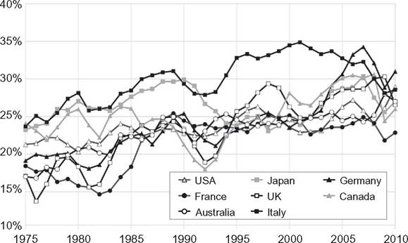
Figure 15.25 Capital shares in factor-price national income, 1975-2010.

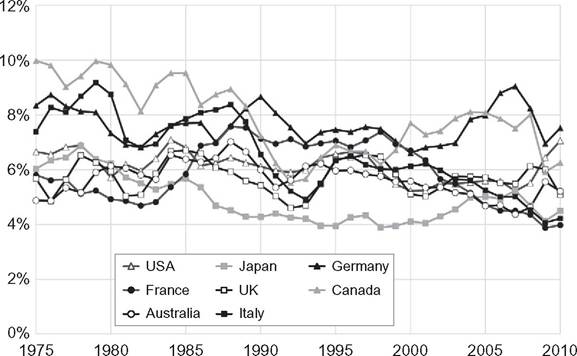
Figure 15.26 Average return on private wealth, 1975-2010.

exactly what one should expect in any economic model: when there is more capital, the rate of return to capital must go down. The interesting question is whether the average return r_t declines less or more than β_t increases. The data gathered by Piketty and Zucman (2014) suggest that r_t has declined less, i.e., that the capital share has increased, consistent with an elasticity σ > 1. This result is intuitive: an elasticity larger than one is what one would expect in a sophisticated economy with different uses for capital (not only land, but also robots, housing, intangible capital, etc.). The elasticity might even increase with globalization, as it becomes easier to move different forms of capital across borders.

Importantly, the elasticity does not need to be hugely superior to one in order to account for the observed trends. With an elasticity σ around 1.2-1.6, a doubling of capital-output ratio β can lead to a large rise in the capital share α. With large changes in β, one can obtain substantial movements in the capital share with a production func­tion that is only moderately more flexible than the standard Cobb-Douglas function. For instance, with σ = 1.5, the capital share rises from α = 28% to α = 36% if the wealth­income ratio jumps from β = 2.5 to β = 5, which is roughly what has happened in rich countries since the 1970s. The capital share would reach α = 42% in case further capital accumulation takes place and the wealth-income ratio attains β = 8. In case the produc­tion function becomes even more flexible over time (say, σ = 1.8), the capital share would then be as large as α = 53%.³⁵ The bottom line is that we certainly do not need to go all the way toward a robot economy (σ = ∞) in order to generate very large move­ments in the capital share.

15.5.4 The Steady-State Level of Wealth Concentration: Ineq = Ineq (r—g) The possibility that the capital-income ratio β—and maybe the capital share α—might rise to high levels entails very different welfare consequences depending on who owns capital. As we have seen in Section 15.3, wealth is always significantly more concentrated than income, but wealth has also become less concentrated since the nineteenth to early twentieth century, at least in Europe. The top 10% wealth holders used to own about 90% of aggregate wealth in Europe prior to World War I, whereas they currently own about 60-70% of aggregate wealth.

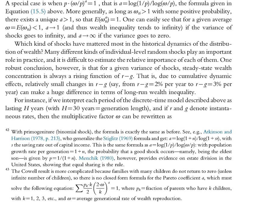
What model do we have to analyze the steady-state level of wealth concentration? There is a large literature devoted to this question. Early references include Champernowne (1953), Vaughan (1979), and Laitner (1979). Stiglitz (1969) is the first attempt to analyze the steady-state distribution of wealth in the neoclassical growth model. In his and similar models of wealth accumulation, there is at the same time both convergence of the macro-variables to their steady-state values and of the distribution of wealth to its steady-state form. Dynamic wealth-accumulation models with random

idiosyncratic shocks have the additional property that a higher r — g differential (where r is the net-of-tax rate of return to wealth and g is the economy’s growth rate) tends to mag­nify steady-state wealth inequalities. This is particularly easy to see in dynamic model with random multiplicative shocks, where the steady-state distribution of wealth has a Pareto shape, with a Pareto exponent that is directly determined by(for a given structure of shocks).

15.5.4.1 An Illustrative Example with Closed-Form Formulas

To illustrate this point, consider the following model with discrete time t = 0, 1,2,.... The model can be interpreted as an annual model (with each period lasting H = 1 year), or a generational model (with each period lasting H = 30 years), in which case saving tastes can be interpreted as bequest tastes. Suppose a stationary population N_t = [0, 1] made of a continuum of agents of size one, so that aggregate and average variables are the same for wealth and national income: W_t = w_t and Y_t = y_t Effective labor input

³⁶ For a class of dynamic stochastic models with more general structures of preferences and shocks, see Piketty and Saez (2013).

In the open-economy case, the world rate of return r_t = r is given. From the above equa­tion one can easily see that β_t converges toward a finite limit β if and only if

id="Picutre 228" class="lazyload" data-src="/files/uch_group77/uch_pgroup315/uch_uch7350/image/image228.jpg">

15.5.4.2 Pareto Formulas in Multiplicative Random Shocks Models

More generally, one can show that all models with multiplicative random shocks in the wealth accumulation process give rise to distributions with Pareto upper tails, whether the shocks are binomial or multinomial, and whether they come from tastes or other fac­tors. For instance, the shock can come from the rank of birth, such as in the primogen­iture model of Stiglitz (1969),42 or from the number of children (Cowell, 1998),4³ or from rates of return (Benhabib et al., 2011, 2013; Nirei, 2009). Whenever the transition equation for wealth can be rewritten so as take a multiplicative form

where ω_ti is an i.i.d. multiplicative shock with mean ω = E(ω_ti) < 1, and ε_ti an additive shock (possibly random), then the steady-state distribution has a Pareto upper tail with coefficient a, which must solve the following equation:

15.5.4.3 On the Long-Run Evolution ofr—g

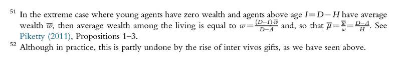
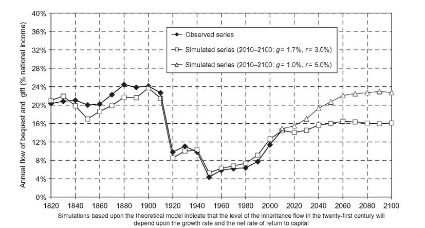
The fact that steady-state wealth inequality is a steeply increasing function of r — g can help explain some of the historical patterns analyzed in Section 15.3.

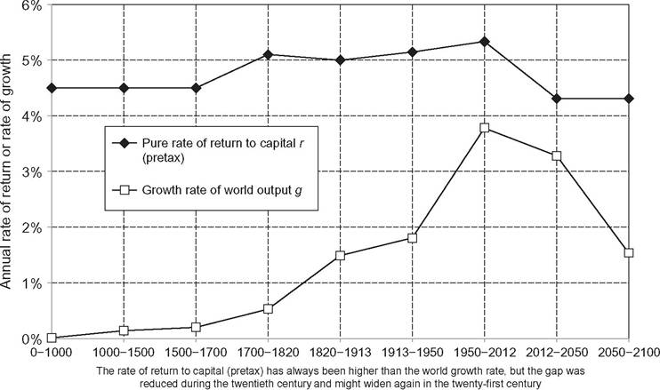
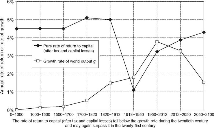
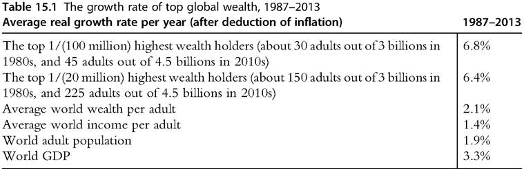
First, it is worth emphasizing that during most of history, the gap r — g was large, typ­ically of the order of 4—5% per year. The reason is that growth rates were close to zero until the industrial revolution (typically less than 0.1-0.2% per year), while the rate of return to wealth was generally of the order of 4-5% per year, in particular for agricultural land, by far the most important asset.^{[48] [49] We have plotted on Figure 15.27 the world GDP growth rates since Antiquity (computed from Maddison, 2010) and estimates of the aver­age return to wealth (from Piketty, 2014). Tax rates were negligible prior to the twen­tieth century, so that after-tax rates of return were virtually identical to pretax rates of return, and the r — g gap was as large as the r — g gap (Figure 15.28).}

The very large r — g gap until the late nineteenth to early twentieth century is in our view the primary candidate explanation as to why the concentration of wealth has been so large during most of human history. Although the rise of growth rates from less than 0.5% per year before the eighteenth century to about 1-1.5% per year during the eighteenth to

Figure 15.27 Rate of return versus growth rate at the world level, from antiquity until 2100.

Figure 15.28 After tax rate of return versus growth rate at the world level, from antiquity until 2100.

nineteenth centuries was sufficient to make a huge difference in terms of population and living standards, it had a relatively limited impact on the r — g gap: r remained much big­ger than £.46

The spectacular fall of the r — g gap in the course of the twentieth century can also help understand the structural decline of wealth concentration, and in particular why wealth concentration did not return to the extreme levels observed before the World Wars. The fall of the r — g gap during the twentieth century has two components: a large rise in g and a large decline in r. Both, however, might well turn out to be temporary.

Start with the rise in g. The world GDP growth rate was almost 4% during the second half of the twentieth century. This is due partly to a general catch up process in per capita GDP levels (first in Europe and Japan between 1950 and 1980, and then in China and other emerging countries starting around 1980-1990), and partly to unprecedented pop­ulation growth rates (which account for about half of world GDP growth rates over the past century). According to UN demographic projections, world population growth rates should sharply decline and converge to 0% during the second half of the twenty- first century. Long run per capita growth rates are notoriously difficult to predict: they might be around 1.5% per year (as posited on Figure 15.27 for the second half of the twenty-first century), but some authors—such as Gordon (2012)—believe that they could be less than 1%. In any case, it seems plausible that the exceptional growth rates of the twentieth century will not happen again—at least regarding the demographic component—and that g will indeed gradually decline during the twenty-first century.

Looking now at r, we also see a spectacular decline during the twentieth century. If we take into account both the capital losses (fall in relative asset prices and physical destructions) and the rise in taxation, the net-of-tax, net-of-capital-losses rate of return r fell below the growth rate during the entire twentieth century after World War I.

Other forms of capital shocks could occur in the twenty-first century. But assuming no new shock occurs, and assuming that rising international tax competition to attract capital leads all forms of capital taxes to disappear in the course of the twenty-first century (arguably a plausible scenario, although obviously not the only possible one), the net-of- tax rate of return r will converge toward the pretax rate of return r, so that the r — g gap will again be very large in the future. Other things equal, this force could lead to rising wealth concentration during the twenty-first century.

The r — g gap was significantly larger in Europe than in the United States during the nineteenth century (due in particular to higher population growth in the New World). This fact can contribute to explain why wealth concentration was also higher in Europe. The r — g gap dramatically declined in Europe during the twentieth century—substantially more than the United States, which can, in turn, explain why wealth has become structurally less concentrated than in the United States. The higher level of labor income inequality in the United States in recent decades, as well as the sharp drop in tax progressivity, also contribute to higher wealth concentration in the United States (see Saez and Zucman, 2014). Note, however, that the United States is still characterized by higher population growth (as compared to Europe and Japan), and that this tends to push in the opposite direction (i.e., less wealth concentration). So whether the wealth inequality gap with Europe will keep widening in coming decades is very much an open issue at this stage.

More generally, we should stress that although the general historical pattern of r — g (both over time and across countries) seems consistent with the evolution of wealth con­centration, other factors do also certainly play an important role in wealth inequality.

One such factor is the magnitude of idiosyncratic shocks to rates of return r_ti, and the possibility that average rates of return r(w) = E(r_ti∖w_ti = w) vary with the initial wealth levels. Existing evidence on returns to university endowments suggests that larger endowments indeed tend to get substantially larger rates of returns, possibly due to scale economies in portfolio management (Piketty 2014, Chapter 12). The same pattern is found for the universe of U.S. foundations (Saez and Zucman, 2014). Evidence from Forbes global wealth rankings also suggests that higher wealth holders tend to get higher returns. Over the 1987—2013 period, the top fractiles (defined in proportion to world adult population) of the Forbes global billionaire list have been growing on average at about 6-7% per year in real terms, when average adult wealth at the global level was rising at slightly more than 2% per year (see Table 15.1).

Whatever the exact mechanism might be, this seems to indicate that the world dis­tribution of wealth is becoming increasingly concentrated, at least at the top of the dis­tribution. It should be stressed again, however, that available data is of relatively low quality. Little is known about how the global wealth rankings published by magazines

Between 1987 and 2013, the highest global wealth fractiles have grown at 6-7% per year, versus 2.1% for average world wealth and 1.4% for average world income. All growth rates are net of inflation (2.3% per year between 1987 and 2013).

are constructed, and it is likely that they suffer from various biases. They also focus on such a narrow fraction of the population that they are of limited utility for a compre­hensive study of the global distribution of wealth. For instance, what happens above $1 billion does not necessarily tell us much about what happens between $10 and 100 million. This is a research area where a lot of progress needs to be made.

15.5.5 The Steady-State Level of the Inheritance Share:

15.5.5.1 The Impact of Saving Motives, Growth, and Life Expectancy

The return of high wealth-income ratios β does not necessarily imply the return of inher­itance. From a purely logical standpoint, it is perfectly possible that the steady-state β = s/g rises (say, because g goes down and s remains relatively high, as we have observed in Europe and Japan over the recent decades), but that all saving flows come from life­cycle wealth accumulation and pension funds, so that the inheritance share φ is equal to zero. Empirically, however, this does not seem to be the case. From the (imperfect) data that we have, it seems that the rise in the aggregate wealth-income ratio β has been accompanied by a rise in the inheritance share φ, at least in Europe.

This suggests that the taste for leaving bequests (and/or the other reasons for dying with positive wealth, such as precautionary motives and imperfect annuity markets) did not decline over time. Empirical evidence shows that the distribution of saving motives varies a lot across individuals. It could also be that the distribution of saving motives is partly determined by the inequality of wealth. Bequests might partly be a luxury good, in the sense that individuals with higher relative wealth also have higher bequest taste on average. Conversely, the magnitude of bequest motives has an impact on the steady-state level of wealth inequality. Take, for instance, the dynamic wealth accumu­lation model described above. In that model we implicitly assume that individuals leave wealth to the next generation. If they did not, the dynamic cumulative process would start at zero all over again at each generation, so that steady-state wealth inequality would tend to be smaller.

Now, assume that we take as given the distribution of bequest motives and saving parameters. Are there reasons to believe that changes in the long-run growth rate g or in the demographic parameters (such as life expectancy) can have an impact on the inher­itance share φ in total wealth accumulation?

This question has been addressed by a number of authors, such as Laitner (2001) and DeLong (2003).⁴⁷ According to DeLong, the share of inheritance in total wealth accu­mulation should be higher in low-growth societies, because the annual volume of new savings is relatively small in such economics (so that in effect most wealth originates from inheritance). Using our notations, the inheritance share φ = φ(g) is a decreasing function of the growth rate g.

47

See also Davies et al. (2012, pp. 123-124).

This intuition is interesting (and partly correct) but incomplete. In low-growth soci­eties, such as preindustrial societies, the annual volume of new savings—for a given

This intuition, however, is incomplete, for two reasons. First, as we already pointed out in Section 15.4, saving flows partly come from the return to inherited wealth, and this needs to be taken into account. Next, the μ parameter, i.e., the relative wealth of dece­dents, is endogenous and might well depend on the growth rate g, as well as on demo­graphic parameters such as life expectancy and the mortality rate m. In the pure life-cycle model where agents die with zero wealth, μ is always equal to zero, and so is the inher­itance share φ, independently of the growth rate g, no matter how small g is. For given (positive) bequest tastes and saving parameters, however, one can show that in steady state, μ = μ(g, m) tends to be higher when growth rates g and mortality rates m are lower.

15.5.5.2 A Simple Benchmark Model of Aging Wealth and Endogenous m

To see this point more clearly, it is necessary to put more demographic structure into the analysis. Here we follow a simplified version of the framework introduced by Piketty (2011).

Consider a continuous-time, overlapping-generations model with a stationary pop­ulation N_t = [0, 1] (zero population growth). Each individual i becomes adult at age a = A, has exactly one child at age a = H, and dies at age a = D. We assume away inter-vivos gifts, so that each individual inherits wealth solely when his or her parent dies, that is, at age a = I = D — H.

Forexample, if A = 20, H = 30, and D = 60, everybody inherits at age I = D — H = 30 years old. But if D = 80, then everybody inherits at age I = D — H = 50 years old.

Given that population N_t is assumed to be stationary, the (adult) mortality rate m_t is also stationary, and is simply equal to the inverse of (adult) life expectancy:

48

It is more natural to focus upon adults because minors usually have very little income or wealth (assuming that I> A, i.e., D — A>H, which is the case in modern societies).

For example, if A = 20 and D = 60, the mortality rate is m = 1/40 = 2.5%. If D = 80, the mortality rate is m = 1/60 = 1.7%. That is, in a society where life expectancy rises from 60 to 80 years old, the steady-state mortality rate among adults is reduced by a third. In the extreme case where life expectancy rises indefinitely, the steady-state mortality rate becomes increasingly small: one almost never dies.

Does this imply that the inheritance flow b_y = μ ∙ m ∙β will become increasingly small in aging societies? Not necessarily: even in aging societies, one ultimately dies. Most importantly, one tends to die with higher and higher relative wealth. That is, wealth also tends to get older in aging societies, so that the decline in the mortality rate m can be compensated by a rise in relative decedent wealth μ (which, as we have seen, has been the case in France).

Assume for simplicity that all agents have on average the same uniform saving rate s on all their incomes throughout their life (reflecting their taste for bequests and other saving motives such a precautionary wealth accumulation) and a flat age-income profile (includ­ing pay-as-you-go pensions). Then one can show that the steady-state μ = μ(g) ratio is given by the following formula:

241" class="lazyload" data-src="/files/uch_group77/uch_pgroup315/uch_uch7350/image/image241.jpg">

In other words, the relative wealth of decedents μ(g) is a decreasing function of the growth rate g (and an increasing function of the rate of return r or of the capital share α). If one introduces taxes into the model, one can easily show that μ is a decreasing function of the growth rate g and an increasing function of net-of-tax rate of return r (or the net- of-tax capital share α).⁵⁰

The intuition for this formula, which can be extended to more general saving models, is the following. With high growth rates, today’s incomes are large as compared to past incomes, so the young generations are able to accumulate almost as much wealth as the older cohorts, in spite of the fact that the latter have already started to accumulate in the past, and in some cases have already received their bequests. Generally speaking, high growth rates g are favorable to the young generations (who are just starting to accumulate wealth, and who therefore rely entirely on the new saving flows out of current incomes), and tend to push for lower relative decedent wealth μ. High rates of return r, by contrast,

are more favorable to older cohorts, because this makes the wealth holdings that they have accumulated or inherited in the past grow faster, and tend to pusher for higher μ.

In the extreme case where g → ∞, then μ → 1 (this directly follows from flat saving rates and age-labor income profiles).

15.5.5.3 Simulating the Benchmark Model

Available historical evidence shows that the slowdown of growth is the central economic mechanism explaining why the inheritance flow seems to be returning in the early twenty-first century to approximately the same level b_y ≈ 20% as that observed during the nineteenth and early twentieth centuries.

By simulating a simple uniform-saving model for the French economy over the 1820—2010 period (starting from the observed age-wealth pattern in 1820, and using observed aggregate saving rates, growth rates, mortality rates, capital shocks and age-labor

Figure 15.29 Observed and simulated inheritance flow, France 1820-2100.

income profiles over the entire period), one can reasonably well reproduce the dynamics of the age-wealth profile and hence of the μ ratio and the inheritance flow b_y over almost two centuries (see Figure 15.29).

We can then use this same model to simulate the future evolution of the inheritance flow in coming decades. As one can see on Figure 15.29, a lot depends on future values of the growth rate g and the net-of-tax rate of return r over the 2010-2100 period. Assum­ing g = 1.7% (which corresponds to the average growth rate observed in France between 1980 and 2010) and r = 3.0% (which approximatively corresponds to net-of-tax average real rate of return observed in 2010), then b_y should stabilize around 16-17% in coming decades. Ifgrowth slows g = 1.0% and the net-of-tax rate of return rises to r = 5.0% (e.g., because of a rise of the global capital share and rate of return, or because of a gradual repeal of capital taxes), b_y would keep increasing toward 22-23% over the course of the twenty- first century. The flow of inheritance would approximately return to its nineteenth and early twentieth centuries level.

In Figure 15.30, we use these projections to compute the corresponding share φ of cumulated inheritance in the aggregate wealth stock (using the PPVR definition and the same extrapolations as those described above). In the first scenario, φ stabilizes around 80%; in the second scenario, it stabilizes around 90% of aggregate wealth.

These simulations, however, are not fully satisfactory, first because a lot more data should be collected on inheritance flows in other countries, and next because one should ideally try to analyze and simulate both the flow of inheritance and the inequality of

Figure 15.30 The share of inherited wealth in total wealth, France 1850-2100.

wealth. The computations presented here assume uniform saving and solely attempt to reproduce the age-average wealth profile, without taking into account within-cohort wealth inequality. This is a major limitation.

15.6.