Axiomatic Measures
The axiomatic approach to multidimensional poverty measurement refers to measures that, given their mathematical structure, satisfy principles or axioms—in other words, behave in predictable ways.
Chapter 2 introduced and discussed the various properties proposed in the literature on multidimensional poverty measurement and their normative justification. We observed that no measure can satisfy all axioms because some of them formally conflict. This section briefly surveys key multidimensional poverty measures that have been proposed and the different subsets of those properties each satisfies. The decision of which measure to choose often distils into a discussion of which axiom sets are more desirable. To blend this assessment with feasibility considerations, we follow Alkire and Foster (2013) in introducing indicator scales of measurement into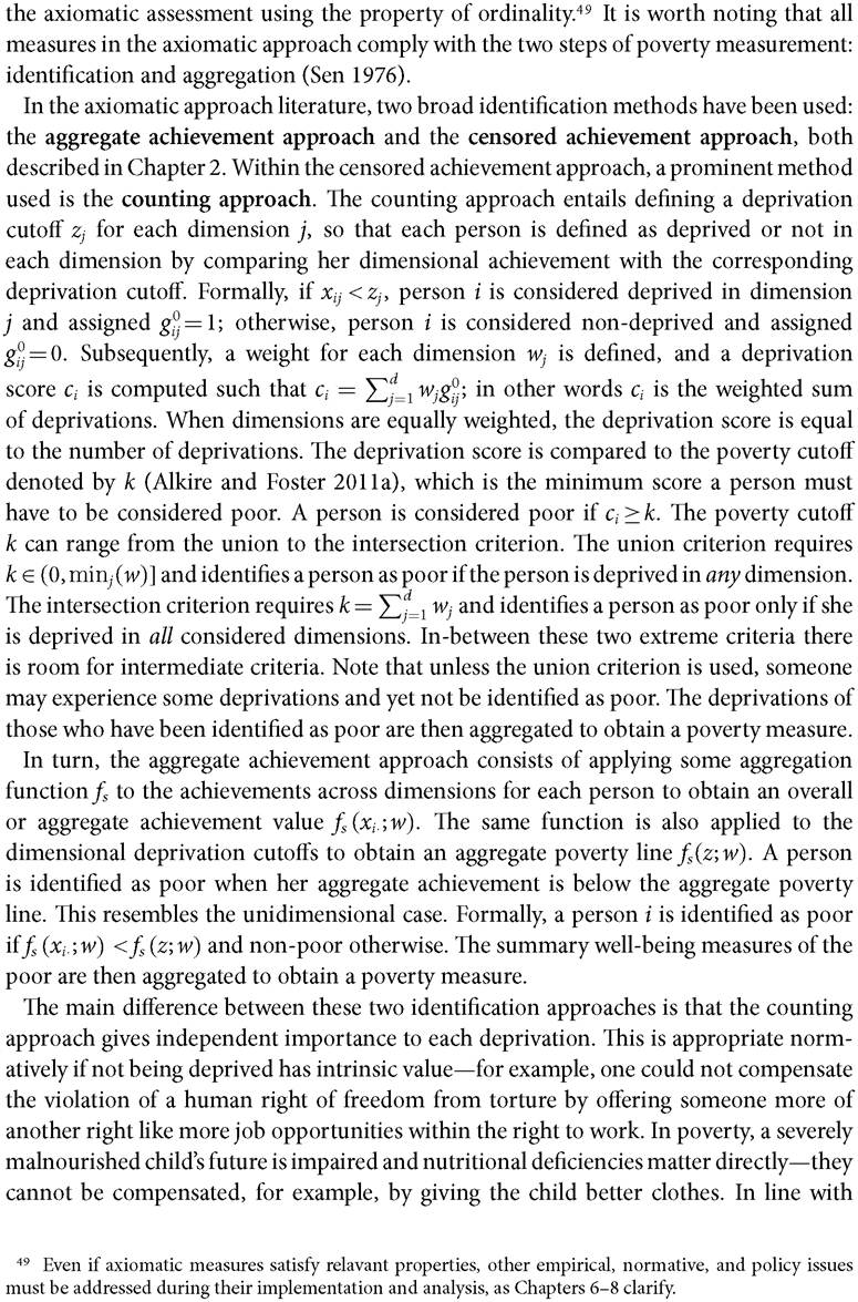
these requirements a counting approach does not allow a non-deprived dimension to compensate for a deprived dimension, whereas the aggregate achievement approach allows such compensation. Thus, the aggregate achievement approach can violate the deprivation-focus property.
Before we present the different measures proposed within each identification method, let us introduce the most basic measure that has been used in the multidimensional context: the multidimensional headcount ratio.50 This measure can be used with different identification methods. Recall that q is the number of people who have been identified as poor, regardless of the identification method used—that is, all people i such that i ∈ Z. The multidimensional headcount ratio is given by
In other words, the headcount ratio, or incidence of poverty, is the proportion of the population who have been identified as poor.
The headcount ratio applies to indicators of any scale type. It satisfies symmetry, replication invariance, scale invariance, poverty focus, and, depending on the identification method used, may also satisfy deprivation focus. In addition, it satisfies weak dimensional monotonicity, weak monotonicity, weak transfer, and weak rearrangement. However, it does not satisfy any of the strong versions of the previous properties. It is fully subgroup decomposable, but, importantly, it does not satisfy dimensional breakdown and continuity.3.6.1 MEASURES BASED ON A COUNTING APPROACH
50 See Chapter 4 for examples of uses of the headcount ratio alongside counting approaches to identify the poor in the multidimensional context.
51 See section 2.3 for a discussion on scales of measurement.
the further the deprived achievements are beneath the deprivation cutoff. Note that for any non-deprived achievement, Xij = Zj, and naturally gij = 0. The value taken by α depends on the kind of dominance properties—monotonicity or transfer—that must be satisfied.
In what follows, we classify the measures that use a counting approach for identifying the poor according to the property of ordinality, beginning with those which can only be implemented when all indicators are cardinal, then turning to those which permit indicators of an ordinal nature.
3.6.1.1 Measures Applicable to Cardinal Variables
Let us first present key multidimensional poverty measures that employ a counting approach to identification, use the union criterion, and assume the underlying variables to be cardinal. The earliest axiomatic multidimensional measures were proposed by Chakravarty, Mukherjee, and Ranade (1998) and are defined in a general way as
where f is continuous, non-increasing, and convex such that f (0) = 1 and f (1) = 0.
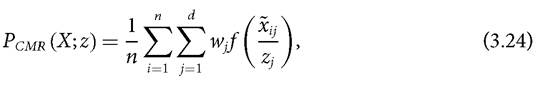
Note that f (1) is obtained when xij = zj, which means that person i is not deprived in dimension j. On the other hand, f (0) is obtained when xij = 0. The measure satisfies many of the properties introduced in section 2.5. In particular, Pcmr satisfies symmetry, replication invariance, scale invariance, poverty focus, deprivation focus, weak monotonicity, dimensional monotonicity, weak transfer, weak deprivation rearrangement, population subgroup decomposability, dimensional breakdown, normalization, non-triviality, and continuity. However, the measure does not satisfy the strong deprivation rearrangement property.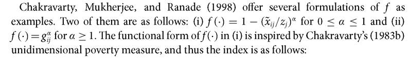
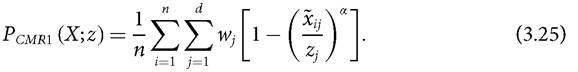
Note that for α = 1, Pcmr1 = Pcmr2, being the average normalized deprivation gap across dimensions and across people.
The class of indices Pcmr was designed to satisfy the dimensional breakdown property. As discussed in section 2.5, this property is incompatible with strong versions of rearrangement properties (Alkire and Foster 2013). Other measures have been designed to be sensitive to associations between dimensions. For example, Tsui (2002) proposed two different classes of multidimensional indices of poverty. One is based on the unidimensional measure proposed by Chakravarty (1983b). The other is based on the unidimensional index proposed by Watts (1968).[116] The first class of indices is defined as
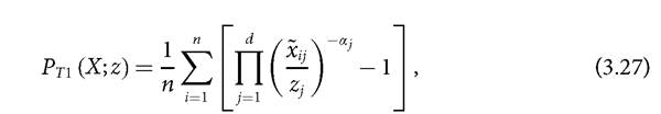
where αj ≥ O for all j and the αjs have to be chosen so that ∏jL 1 [χij/zj) 'α is convex in its arguments.
The requirement of convexity is to guarantee that the measure satisfies the transfer principle stated in section 2.5.2. PT1 satisfies symmetry, replication invariance, scale invariance, poverty focus, deprivation focus, weak monotonicity, dimensional monotonicity, weak transfer, weak deprivation rearrangement (assuming achievements to be substitutes), population subgroup decomposability, and continuity. It does not satisfy dimensional breakdown and normalization because the maximum value is not bounded by 1; however, the measure is bounded at 0, i.e. PT1 = 0 whenever there is no one who is poor in the society. PT1 satisfies non-triviality when at least one α,j > 0 and strong deprivation rearrangement when αj > 0 for all j.The second family of indices proposed by Tsui (2002) is given by
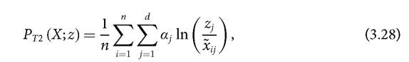
invariance, scale invariance, poverty focus, deprivation focus, weak monotonicity, dimensional monotonicity, weak transfer, weak deprivation rearrangement, population subgroup decomposability, dimensional breakdown, and continuity. However, the measure does not satisfy the property of strong deprivation rearrangement. The property of normalization is not satisfied because its upper bound is not equal to one.
The next two classes of multidimensional poverty indices were proposed by Bour- guignon and Chakravarty (2003). The first class of indices is a straightforward extension of the unidimensional family of indices by Foster, Greer, and Thorbecke (1984). The class of measures is defined as follows:
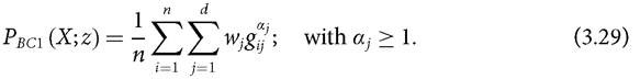
By design, the class of indices in (3.29) is identical to the class of indices in (3.26) and so satisfies identical properties. Bourguignon and Chakravarty (2003) extended Tsui (2002), in terms of the sensitivity of a poverty index to association between dimensions, to the case in which achievements can be considered complements.
The second class of measures proposed by Bourguignon and Chakravarty is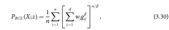
measures proposed by Alkire and Foster (2007,2011a) can be expressed as
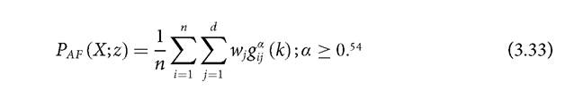
All measures in the Paf family satisfy symmetry, replication invariance, scale invariance, poverty focus, deprivation focus, dimensional monotonicity, population subgroup decomposability, dimensional breakdown, and weak deprivation rearrangement. For
3.6.1.2 Measures Applicable to Ordinal Variables 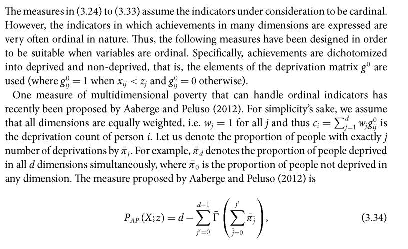

[1] Silber and Yalonetzky (2013) have presented the Aaberge and Peluso measure by dividing by the total number of dimensions d so that the measure lies between 0 and 1.
poverty focus, deprivation focus, ordinality, dimensional monotonicity, weak deprivation rearrangement, normalization, and subgroup consistency. It does not satisfy the axioms of population subgroup decomposability and dimensional breakdown.
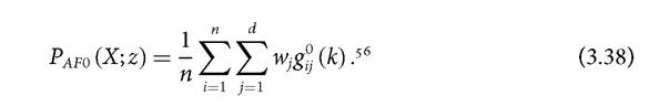
Finally, it should be emphasized that one of the measures of the AF family introduced in the previous section is suitable for ordinal variables—the Adjusted Headcount Ratio. Following (3.33), the measure can be expressed as
This measure satisfies symmetry, replication invariance, scale invariance, poverty focus, deprivation focus, ordinality, dimensional monotonicity, weak monotonicity, normalization, non-triviality, weak rearrangement, population subgroup decomposability, and dimensional breakdown.
However, it does not satisfy monotonicity, weak transfer and strong rearrangement. Note that the Paf0 measure coincides with both Pcdi and Pbcd for β = 1, when a union criterion is used for identifying the poor (see Chapter 5).It is worth noting that, like the multidimensional headcount ratio in (3.23), the measures (3.34) to (3.38) are suitable for ordinal variables, but they are also superior to measure (3.23) because they satisfy dimensional monotonicity. Additionally, the Adjusted Headcount Ratio in (3.38) satisfies the dimensional breakdown property.
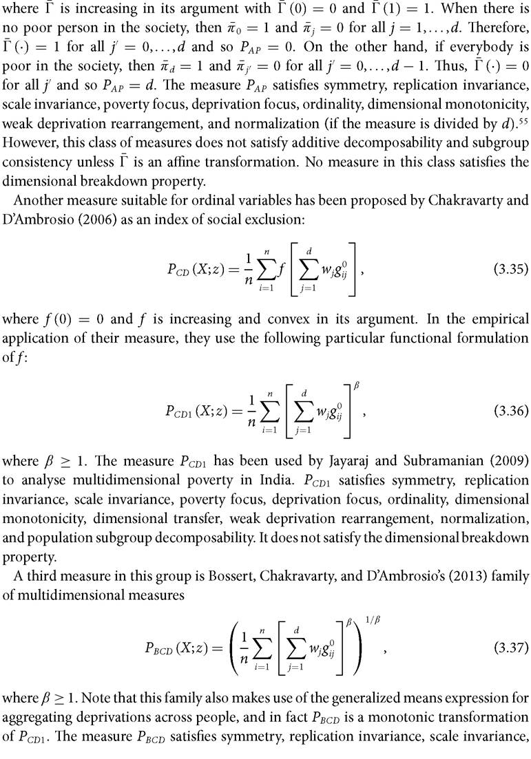
3.6.2 MEASURES USING AN AGGREGATE ACHIEVEMENT APPROACH
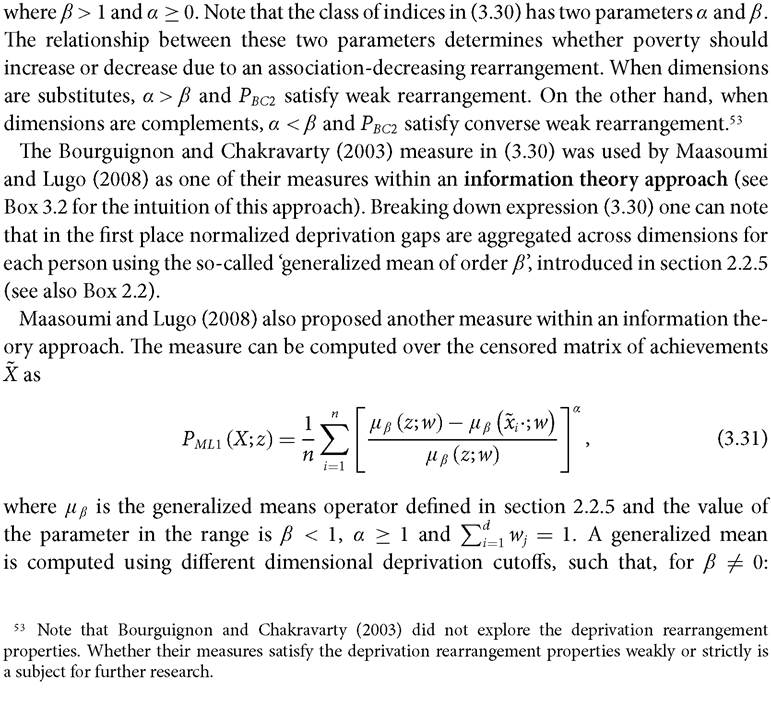
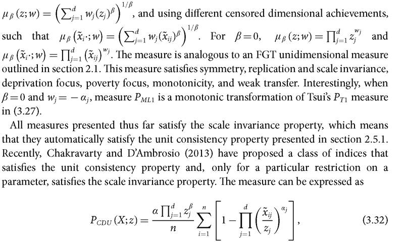
In the aggregate achievement line approach, we find one measure developed by Maasoumi and Lugo (2008) within the so-called information theory approach (see Box 3.2).[117] It is should be observed that these measures require indicators to be cardinal. The measure is defined as follows:

[1] Alkire and Foster (2011a) use the notation ‘M0’ to denote the Adjusted Headcount Ratio, which is used from Chapter 5 onwards. In order to preserve uniformity in the use of notation across this chapter, we use the notation Paf0.
BOX 3.2 INFORMATION THEORY MEASURES
Maasoumi and Lugo's (2008) multidimensional poverty measures emerged from the so-called information theory approach. The approach is called 'information theory' because it borrows from measures of information related to event occurrences in the context of engineering (Shannon 1948). The approach is built around three main concepts: (1) information content, (2) measurement of entropy, and (3) measurement of entropy divergence or relative entropy between two probability distributions.
(1) Information content: Suppose one has a set of possible events, each of which has an associated probability of occurrence. The information content that a certain event has occurred is greater the lower its probability of occurrence is. In other words, the information content of the occurrence of an event is inversely related to its probability of occurrence. If the event was very likely to occur, then the information that it has occurred is not very interesting, as this was highly expected. On the contrary, if the event was unlikely, the information that it has occurred is indeed very interesting.
(2) Measure of entropy: Given an experiment with n possible outcomes, entropy is defined as the expected information content—that is, the sum of the information content of each event weighted by its probability. Entropy can be understood as a measure of uncertainty, disorder, or volatility associated with a distribution (Maasoumi 1993: 141). The more concentrated the probability of occurrence around one event is, the lower entropy will be: that is, the lower will be the expected information content from those possible outcomes as one particular outcome is highly predicted. On the other hand, when all events are equally likely to occur, entropy is higher: that is, the expected information content from those possible outcomes will be higher as no particular outcome is highly predicted; thus, there is a lot of uncertainty.
(3) Measure of entropy divergence or relative entropy: Given two probability distributions, a measure of entropy divergence or relative entropy between them assesses how the two distributions differ from each other (Kullback and Leibler 1951).
The concepts of information theory were first used in distributional analysis in order to measure income inequality by Theil (1967). Consider an income (achievement) distribution x with n incomes. Here each particular income value is an 'event'. The distribution of income shares, where each share is given by —,
/=1 xi can be interpreted as a probability distribution. If all incomes are obtained by only one person (i.e. one share equals 1 and the rest equal 0), this is the situation of lowest entropy. Undoubtedly, it is also the situation
BOX 3.2 (cont.)
of highest inequality. On the other hand, if every person receives the same share of income (1 /n), this is the situation of highest entropy. Undoubtedly, it is also the situation of lowest inequality. Thus, inequality can be seen as the complement of entropy. Equivalently, a measure of inequality can be constructed using a measure of entropy divergence, where inequality is given by the distance between the probability distribution of a perfectly equal distribution (each probability being 1/n) and the actual observed income distribution (each probability being the actual income share of each person). Theil proposed two measures of income inequality which are essentially the minimum possible distance between an 'ideal' distribution (perfectly equal) and the one observed (Maasoumi and Lugo 2008).
Although not easily interpretable, Theil indices became attractive measures of inequality because they satisfy four properties considered to be essential to inequality measurement (Atkinson 1970; Foster 1985; Foster and Sen 1997) and are also additively decomposable, meaning that they can be expressed as a weighted sum of the inequality values calculated for population subgroups (within-group inequality) plus the contribution arising from differences between subgroup means (Shorrocks 1980: 613). Given their attractive characteristics, these measures were extended by Shorrocks (1980), Cowell (1980), and Cowell and Kuga (1981) into a parametric family named 'generalized entropy (GE) measures'.
It is worth emphasizing that the expressions of the generalized means (as described in section 2.2.5) are closely linked to information theory measures. In fact, it is found that the expression of the generalized means is such that it minimizes the entropy divergence or relative entropy between two distributions (Maasoumi 1986; Maasoumi and Lugo 2008).
3.6.3 Acriticalevaluation
Axiomatic measures present a number of convenient features. First, they comply with the two necessary steps of poverty measurement: identifying the poor and aggregating the information into a single headline figure. Second, the portfolio of axiomatic measures includes measures that only apply when indicators are cardinal but also includes measures that apply when indicators are ordinal. Third, the axiomatic measures described in this section, unlike dashboards and composite indices, can use the joint distribution of achievements both at the identification and at the aggregation step. Measures that use a counting approach with the union criterion to identify the poor do not incorporate joint deprivations at the identification step. However, such measures could be implemented with a different criterion requiring joint deprivations as a restriction. In terms of aggregation, only the headcount ratio of multidimensional poverty is insensitive to the joint distribution; the other measures satisfy dimensional monotonicity, and some of them also satisfy the strict versions of rearrangement properties.
A fourth advantage of axiomatic measures is that it is possible to know exactly how they behave under different transformations of the data. Thus, policymakers and researchers can select a particular measure based on the properties it satisfies as well as on its data requirements, namely, whether it requires variables to be cardinal. As mentioned when introducing the properties in section 2.5, some properties are incompatible: a measure can satisfy one or the other but not both, i.e. there is a trade-off. The key decision among feasible axiomatic measures is which properties are to be privileged.
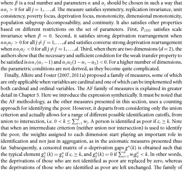
For example, in the presence of cardinal variables, one may want to privilege dimensional breakdown and thus select a measure from the Alkire and Foster (2011a) family of measures. Alternatively, one may want to privilege sensitivity to associations among dimensions (strong rearrangement), foregoing dimensional breakdown, and thus select the Pbc2 measure of the Bourguignon and Chakravarty (2003) family or the Pti measure proposed by Tsui (2002). At the same time, it is also clear that as long as one of the considered dimensions is measured with an ordinal indicator, the set of applicable measures is substantially reduced but the practicality is greatly expanded, so again decisions need to be made. If one is not concerned about capturing the intensity of deprivations (dimensional monotonicity), the headcount ratio of multidimensional poverty will work. On the contrary, if one wants a measure that is sensitive to intensity and provides policy incentives to address those with high deprivation scores, one can select the Paf0 measure of the Alkire and Foster (2011a) family, the Pbcd measure proposed by Bossert, Chakravarty, and DAmbrosio (2013), or the Pcdi measure proposed by Chakravarty and DAmbrosio (2OO6). However, if one would like the measure to satisfy dimensional breakdown as well, then neither the Pbcd measure nor the Pcdi measure are suitable—although Paf0 is. Note that these types of decisions regarding the trade-offs between certain properties are not minor issues as they have direct implications for policy design and assessment. Ultimately, these decisions reflect the properties that the researcher or policymaker holds to be so important that they should be axioms—that is, undisputable attributes a measure must exhibit.
Constructing measures based on axiomatic properties has several merits. First, for any poverty index, it is important to understand how the measure behaves with respect to various data transformations. A measure that does not satisfy certain properties understood to be fundamental—say, weak monotonicity—may lead to dire policy consequences. Despite the advantages of axiomatic poverty measures, they also have limitations—as is true for any measurement methodology. First, for the reasons already stated, no single measure can satisfy all the properties presented in Chapter 2 at the same time. Thus, the selection of one measure over others always involves normative trade-offs. Yet, as long as such action is explicit and justifications are provided, by no means should this discourage the use of axiomatic measures. Second, the measures presented in this section require data to be available from the same source for each unit of identification. This may reduce the applicability of these measures when it is not possible to obtain such data. Yet, as data collection continues to improve, this difficulty will be progressively eased. Third, as mentioned at the end of the dominance approach section, axiomatic measures might be criticized for providing a complete ordering and cardinally meaningful distances between poverty values at the cost of imposing an arbitrary structure. However, not only are these properties desirable from a policy and practical perspective, but axiomatic measures are transparent about the structure they impose.
Despite these limitations, we take the view that axiomatic measures offer a strong tool for measuring multidimensional poverty, with the advantages outweighing the potential
Table 3.2 Summary of the multidimensional poverty measurement methodologies
| Method | Able to capture joint distribution of deprivations: require microdata | Identification of the poor | Provide a single cardinal index to assess poverty |
| Dashboards | No | No | No |
| Composite Indices | No | No | Yes |
| Venn Diagrams | Yes | May | No |
| Dominance Approach | Yes | Yes | No |
| Statistical Approaches | Yes | May | May |
| Fuzzy Sets | Yes | Yes | Yes |
| Axiomatic Approaches | Yes | Yes | Yes |
Note: 'May' means that the Compliancewith that criterion depends on the particular technique used within that approach.
drawbacks. Yet many of the other methodologies for poverty measurement addressed throughout this chapter can work as invaluable complementary tools, as we shall see.
This chapter provides an overview of methodologies that are used for multidimensional poverty measurement or analysis other than the counting approach, to which we shall shortly turn. The chapter has described the main characteristics, scopes, and limitations of these methodologies. Table 3.2 presents a schematic summary of the reviewed methodologies in terms of three essential characteristics, namely: whether the methodology is able to capture the joint distribution of deprivations, whether it identifies the poor (i.e. dichotomizing the population into poor and non-poor, creating the set of the poor), and whether it provides a single cardinal figure to assess poverty.
Many methodologies outlined in this chapter rely on the assumption that data for all dimensions are cardinal. Others are applied to ordinal data, but make strong assumptions that the ordinal information can be treated as cardinal equivalent. Poverty measures based on the counting approach, however, do not make such assumptions and satisfy the ordinality property. Chapters 5-10 focus on a particular poverty measurement methodology proposed by Alkire and Foster (2011), that is based on a counting approach. Before introducing this particular poverty measurement methodology, we step back in Chapter 4 to present a historical review of applications of the counting approach to identify the poor and the ways it has been used in different parts of the world.