EARNINGS DISTRIBUTION AND INCOME DISTRIBUTION: A SHORT TALE OF TWO LONG LITERATURES
In spite of recent declines in the labor share in GDP or national income,[115] the income that people generate in the labor market is obviously the most frequent and most important
part ofhousehold incomes, and the inequality oflabor earnings seems an important determinant ofincome inequality at face value.
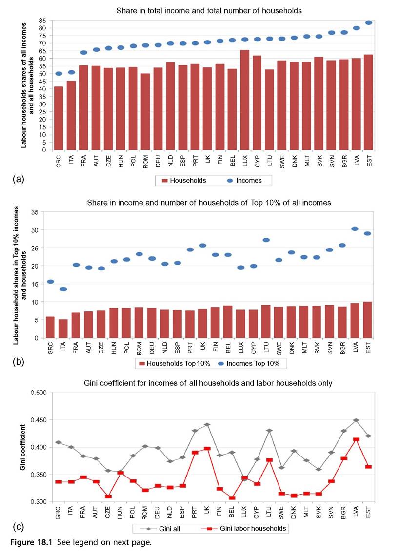
Figure 18.1 portrays in three panels the role of “labor households,” which are defined as households receiving more than half their total income from wage earnings, across 26 countries ofthe European Union. Panel (a) ranks the countries by the income share of labor households (the markers), and the same ranking is adopted for the other panels. Panel (a) indicates that labor households receive the majority of all incomes, ranging from slightly over 50% in Greece and Italy up to a maximum of 84% in Estonia. They comprise significantly smaller shares of all households, however, ranging from less than half in Greece and Italy[116] to 66% in Luxembourg. Clearly, these households’ mean incomes are above average in all countries. This is borne out by panel (b), which indicates similar shares with a focus on the Top 10% of all incomes in a country. The income share always exceeds the household share and does so by far: on average the income share is 14% points higher than the household share. This contrast with the Bottom 90% (not shown): here the gaps between the two shares are modest, and they can be positive as well as negative; the resulting cross-country average is almost nil. At the same time, in panel (c), the Gini coefficients for all households always exceed that for labor households and they move in striking parallel in various countries characterized by high labor-income inequality such as the United Kingdom, Portugal, Lithuania, Bulgaria, Latvia, and Estonia (overall correlation is 0.75). The Gini levels do not follow the smooth ranking of increasing income shares but vary substantially (correlation 0.23). Therefore, rather dissimilar Gini coefficients can go together with very similar income shares as the middle group, ranging from Germany to Belgium, as illustrated (panel c vs. a). However, for labor households income shares in the Top 10% and the Gini coefficient show a more similar pattern (panel c compared to panel b) (correlation 0.56). So income from labor is highly important indeed, but its effects on income inequality show significant variation and warrant further scrutiny.Another measure of inequality, the income share of the top decile of the distribution, tells basically the same story for all incomes as the Gini and the top share are highly correlated (0.91) (compare Leigh, 2009). However, the gap between all incomes and labor incomes is more substantial here—the correlation of the two top shares is only 0.32—and suggests that the role of high levels of household earnings differs significantly between countries. The linkage between the dispersion of wages and the income distribution is clearly important and also warrants further research.
Though the literature on the two distributions is not absent and perhaps even growing, it is not the subject of a strong strand. Instead, one may surmise, there are two largely separate, extensive literatures, one addressing (individual) wage inequality in the labor market and the other (household) income inequality in society. As Gottschalk and Danziger (2005, 253) observe “Labor economists have tended to focus on changes in the distribution of wage rates, the most restrictive income concept, since they are interested in changes in market and institutional forces that have altered the prices paid to labor of different types. At the other extreme, policy analysts have focused on changes in the distribution of the broadest income concept, family income adjusted for family size. This reflects their interest in changes in resources available to different groups, including the poor.” It confirms that the conclusion drawn 8 years before by Gottschalk and Smeeding (1997, 676), that “an overall framework would simultaneously model the generation of all sources of income...
as well as the formation of income sharing units” and be considered “the next big step that must be taken,” was still a tall order when Gottschalk and Danziger made their contribution. Yet another 5 years later, Jiri Vecernik (2010, 2) observed that “there seems to be a gulf between the analysis of personal earnings and household income.” It seems a foregone conclusion that for the combination of individual wage and earnings inequality and household earnings and income inequality, the unified economic theory of income distribution, hoped for by Atkinson and Bourguignon (2000, 26), is not yet forthcoming though interesting contributions may be found below.[117]This divide has a technical aspect that deserves some attention. The dispersion of wages is commonly conceived as the distribution of hourly wages, i.e., wage rates. The income distribution, by contrast, focuses on annual incomes, and therewith annual earnings, which are the product of hourly wages and annual hours worked. Next to the wage distribution, this brings into play the distribution of hours worked during the year, which, in turn, are the product of jobs and hours on the job. These hours have become a significant dimension of employment in many countries because of the growing importance of part-time employment and temporary jobs. Their presence adds to the traditional effect on annual hours that is exerted by the turnover during the year of people who join or leave employment.[118] As a result we deem it essential to distinguish between various distributions: wages (which are hourly), earnings (which are annual), employment (which concerns annual hours worked), and incomes (which include other sources than earnings).
A second difference is that the wage distribution is commonly conceived in gross terms, that is pretax, whereas on the income side there is a strong focus on disposable incomes—after transfers and taxes—which are often also standardized (equivalized) for the size and composition of the receiving household.[119] The third difference is that the dispersion of wages rests on the individual as the unit of analysis whereas the income distribution is based on the household, which can be a combination of individuals.
Thus, for linking the two distributions, the individuals from the one side need to be linked to their households on the other side. Importantly, this puts the limelight on the distribution of employment and corresponding earnings over households. There is a significant literature on the other side of this employment coin, the nonemployment or joblessness of households, especially in comparison to individual joblessness, which was started by Paul Gregg and Jonathan Wadsworth in the mid-1990s (Gregg et al., 1996, 1998 and Gregg and Wadsworth, 2008). However, this literature is not often linked to the distribution of incomes albeit it may be linked to poverty (De Graaf-Zijl and Nolan, 2011).18.2.1 Individual or Household Incomes?
Before discussing the main points found in the literature we present a few stylized facts that may demonstrate the relevance of considering the link between the two distributions. First, we consider the employment side of the matter. A core message from the joblessness literature is that in many countries individual workless rates have fallen over the past 20 years, but household-based workless rates have not (Gregg et al., 2010, 161). Or to put it the other way around, the growth in (individual) employment-to-population ratios has not been mirrored in a corresponding increase in what can be termed the “household employment rate.” The implication is that much of the additional jobs growth has gone to households already containing a worker. Figure 18.2 illustrates this for a number of European countries since the mid-1990s: most of the decline in individual unemployment has gone to households already engaged in employment and much less has contributed to a lowering of the number of people living in jobless households.
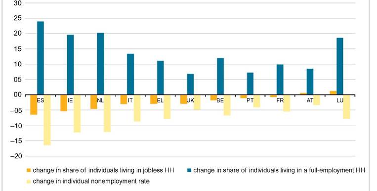
Figure 18.2 Changes (percentage points) in individual and household employment, 11 European countries, 1995-2008. Reading note: In Spain the share among individuals of those in work who are also members of a household where everyone is in work increased by 24% points between 1995 and 2008;the share for those living in households without work declined by 7% points;the share of individuals without work declined by 16.5% points.
Explanatory note: In full-employment households everyone is in work; this includes single-person households. Employment follows the ILO definition and includes the self-employed. Persons aged 18-24 whose status is “inactive” are considered to be full-time students and excluded. For country codes see Appendix A. Source: Eurostat—Corluy and Vandenbroucke, 2013, Figure 1 (based on the European Labour Force Survey).Figure 18.3 adds a particularly sharp example of the divergence between the two rates of employment for prime-age adults for the United Kingdom, one for persons (the traditional individual employment-to-population ratio), the other for households (the percentage of relevant households that have at least one employed person among their members). The former rate always exceeds the latter, and the gap between the two has grown rapidly from 2% points at the end of the 1970s to 13% points since the early 1990s.[120] Often such developments have gone hand in hand with an expansion of part-time employment. The correlation of individuals’ levels of pay to their numbers of hours worked can tell us whether this hours-of-work dimension enhances or mitigates inequality. A positive correlation implies a more unequal distribution of annual earnings than of hourly earnings among individuals. The correlation has tended upward significantly and turned from negative to
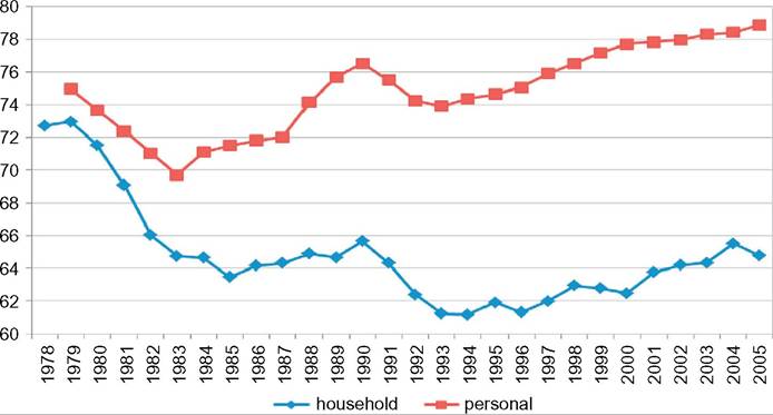
Figure 18.3 Employment rates (%) for individuals aged 25-59 and their households, United Kingdom, 1978-2005. Reading note: The share among individuals aged 25-59 who are in work grew from 75% in 1979 to 79% in 2005;the share of households corresponding to these individuals where at least one person is employed, declined from 73% to 65%. Source: Derived from Blundell and Etheridge (2010), Figures 2.1 and 2.3 (based on Labor Force Survey and Family Expenditure Survey).
positive in some countries although it still is negative in other countries.
The correlation seems particularly strong for British women (Figure 18.4).Compared to single-breadwinner households this complicates the relationship between the wage distribution and the income distribution. At the same time it makes the scrutiny of that relationship all the more important. Thus the role of dual-earner and multiple-earner households has expanded and is now substantial in many European countries as is indicated in Figure 18.5. With the exception of Italy and Greece, dual-earner and multiple-earner households are the majority among households, and evidently, employees in those households make up an even larger share of all employees. In particular, the role of multiple-earner households varies substantially across countries, from 4% of all households in Greece to 27% in Bulgaria.
In a world of full-time-working single-earner households, the correspondence between wage dispersion and income distribution seems pretty straightforward: a high individual wage directly implies a high household income. This traditional situation may provide another explanation, for lack of a problem, why the literature on the linkage between the two distributions seems underdeveloped. The formation of households and their labor supply may affect the distribution of incomes depending on the correlation of earnings levels between the earners in a household. A positive correlation will enhance household earnings inequality, in addition to the frequency of the occurrence of joint earnings. Changes in mating behavior or in partners’ employment participation or both at the same time will be behind this. Figure 18.6 indicates the rise in the correlation
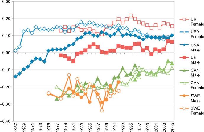
Figure 18.4 Correlation of individual wage level and annual hours worked, by gender, ages 25-59, United States, United Kingdom, Canada and Sweden, 1967-2005. Reading note: The correlation between the annual hours worked and earnings per hour among US males changed from —0.10 in 1967 to +0.10 in 2005. Source: Blundell and Etheridge (2010), Brzozowski et al. (2010), Domeij and Floden (2010), and Heathcote et al. (2010).
between such earners for the United States. It has roughly doubled over 1975-1990, which is less than half the 40-year period, and remained largely stable since. However, the level and evolution of this may differ between countries and, apparently, over time. Conversely, household joint labor supply may also affect the dispersion of wages, if additional earners would operate their labor supply at a less extensive margin of pay or working hours, given that a main income is already secured in the household, or if they would trade off pay and hours for a scenario combining paid labor with other activities, such as household care or participation in education.
In the end, household formation and the two distributions will all be endogenous to each other, and household formation should be added to the list of “stages for comprehending the distribution ofincome: aggregate factor incomes, differences in earnings and in capital incomes, the role of the corporate sector and of financial institutions, and the distributional impact of the state” (Atkinson, 2007a, 20).
18.2.2 A Cursory Review of the Literature Related to Household Incomes Distribution and LMIs
The literature on the linkage between the two distributions is diverse and cannot be viewed yet as a strong and coherent strand. More than occasionally contributions to
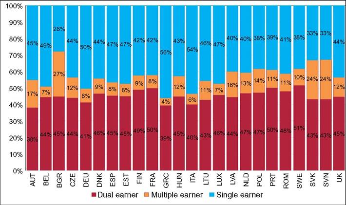
Figure 18.5 Working-age households with employees by number of earners, 26 European countries, 2010. Reading note: In Austria 38% of households with at least one member in employment have two persons employed, 17% have three or more persons employed, and 45% have one person employed (including single-person households). Explanatory note: Earners need to have positive hours and earnings as well. The household main earner is aged below 65, Students as identified in the data set are excluded. Naturally, female employment participation, traditionally large in what are now former communist countries, is an important determinant. Source: Salverda and Haas (2014, Figure 3.9).
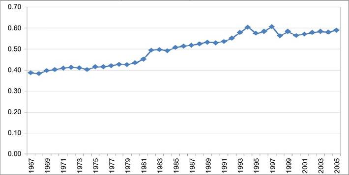
Figure 18.6 Correlation of earnings between married partners, United States, 1967-2005. Reading note: Correlation of earnings levels between married partners in households from less than 0.40 to around 0.60. Source: Heathcote et al. (2010).
the subject are found in papers dedicated to other issues than the income distribution, such as the design of transfer programs (e.g., Liebman, 1998). Our own reading of the literature on household incomes distribution leads us to conclude that it pays little attention to the role of LMIs, which is, after all, the focus of our chapter. This is the very reason that we only touch on the household context of the dispersion of wages here. Checchi and Garcia Peilalosa (2008, 2010) do address LMIs and income inequality. In a comparative cross-country and macroeconomic perspective, they show the relevance of institutions especially in terms of their effects on the level of unemployment (i.e., zero hours and earnings) which, in turn, contributes significantly to the level of income inequality.[121] We will elaborate on elements of their approach later in the chapter. Certainly, some contributions investigate the effects on the income distribution of one particular institution, the minimum wage—itself the subject of a large literature for its effects on the dispersion of wages. Charles Brown (1999, Section 9.2) in his survey of that literature observes that many families have several earners, so that a minimumwage worker can be part of a relatively affluent family and adds that the level of the minimum wage will be of little help in reducing income inequality, basing his argument on simple statistics that show the poor fraction among low-wage workers is low and that many poor families have no workers. Neumark and Wascher (2008) sum up many of their own and other contributions to the minimum-wage literature. In their view the combined evidence of income and employment effects for the United States is best summarized as “indicating that an increase in the minimum wage largely results in a redistribution of income among low-income families” (p. 189), as some may see their income rise and others may see their employment and therewith their income diminish. However, Arindrajit Dube (2013) finds sizable minimum-wage elasticities for the bottom quantiles of the equivalized family income distribution and argues from an evaluation of the existing literature, including works by Neumark and Wascher, that the finding is consistent with that.
There is, however, another emerging literature that studies the role of institutions in connection with the household incomes distribution, especially new institutions of relevance such as parental leave, tax credits, including the American EITC or the British WTC, or entitlements to remain in the same job (e.g., Brewer et al., 2006; Dingeldey, 2001; Dupuy and Fernandez-Kranz, 2011; Eissa and Hoynes, 2004, 2006; Mandel and Semyonov, 2005; Thevenon, 2013; Thevenon and Solaz, 2013; Vlasblom et al., 2001). However, mostly it preoccupies itself with the employment effects and ignores the income side, and it is strongly focused on particular aspects of inequality as, for example, female labor supply or the motherhood gap in employment participation, and does not consider the aggregate picture of inequality nor the effects on earnings inequality or the interrelationship between the two distributions.[122] We leave that literature out here, though we will try in the material to come to incorporate some of those new institutional measures in our broader framework. Note, finally, that we leave out the demographically motivated literature that focuses exclusively on the contribution to income inequality of household structure and composition (e.g., Brandolini and D’Alessio, 2001; Burtless, 2009; Peichl et al., 2010); nevertheless we do include contributions considering this in a broader framework that encompasses earnings inequality (e.g., Burtless, 1999).
10
In the collection of contributions there seem to be two main approaches (see Table 18.A7 in Appendix D for a summary of the relevant literature). The first approach is based on a direct comparison of the different distributions, and the second approach is based on a decomposition ofincome inequality that focuses on the sources ofincome, particularly earnings. The latter shows substantial variation in its choice of the measure of income that is decomposed (mainly established aggregate measures of inequality such as the Gini coefficient, but also newly devised ones such as the “polarization index” designed by Corluy and Vandenbroucke, 2013). [123] More importantly, this literature also varies in the precise technique of decomposition that is applied, which matters as the technique affects the outcome. In the literature there is no single generally accepted way of decomposing, which hampers the establishment of stylized facts.[124] This situation partly motivates the first, comparative approach. In addition to this, it can be observed that the decomposition approach takes one of the two distributions as its starting point and does not consider the effects on the other distribution. Thus it remains unclear when, e.g., growing female employment participation increases household earnings inequality if it also raises individual earnings inequality. We briefly discuss each of the two main approaches.
18.2.2.1 Comparing Distributions
One of the first contributions was made by Gottschalk and Smeeding (1997). They discuss various types of distributions and inequality measures on both the earnings and the income side, but largely in isolation of each other. Their conclusion is that “[b]etter structural models of income distribution and redistribution that can be applied across nations are badly needed. Ideally, an overall framework would simultaneously model the generation of all sources of income (labor income, capital income, private transfers, public transfers, and all forms of taxation) as well as the formation of income sharing units” (p. 676). Thatis still a tall order today. Intheabsenceofsuchaframework, decomposition leaves us with “purely accounting exercises” (p. 668).
Burtless (1999) compares the distributions of annual individual earnings distributions on the one hand and personal equivalized incomes on the other hand for the United States between 1979 and 1996. With the help of simple counterfactual exercises regarding the personal income distribution when holding the levels of earnings inequality constant, he finds that two-thirds of the observed increase in overall income inequality would have occurred leaving only one third for the changes in earnings. Within the latter share he attributes 13% of the increase to the growing correlation between male and female earnings in families. Also the increasing share of single-adult families among the population has contributed because the greater inequality within that group.
Reed and Cancian (2001) also simulate counterfactual distributions for the United States over the period 1969-1999, instead of pursuing a decomposition approach. They argue that this simulation allows using multiple measures of inequality, looking at different points in the distribution, and incorporating changes in the marriage rate. They find that changes in the distribution of female earnings account for most of the growth in family income throughout the distribution and disproportionately more at the bottom, leading to a decrease in inequality. By contrast, changes in male earnings account for over 60% of the growth in the Gini coefficient of the family income distribution.
Gottschalk and Danziger (2005) analyze in an interconnected way the evolution of inequality in four different percentile distributions: hourly individual wage rates, annual individual earnings (and therewith annual hours), annual family earnings, and annual family adjusted total income. The first two distributions are at one side of the earnings-incomes gulf, the other two at the other side. Interestingly, they bridge the gulf by ranking individuals for their annual earnings according to the total earnings of their households (p. 247) using consistent samples of individuals. Earnings exclude the self-employed and the analysis splits throughout between men and women. The focus is the American evolution over the last quarter of the previous century using CPS data.[125]
Atkinson and Brandolini (2006), though, for the most part considering trends in wage dispersion, compare the Gini of the individual annual earnings dispersion to the Gini of adjusted disposable household income for a set of eight countries: Canada, Finland, Germany, the Netherlands, Norway, Sweden, the United Kingdom, and the United States, using LIS data from around the year 2000. They draw the comparison on an annual basis and include part-time and part-year earnings, but they leave the distribution of employment out from their analysis, and, consequently, they also do not compare directly to the hourly wage rates, the traditional pay inequality in the labor market. In addition, they do not compare individuals and households on the basis of an identical ranking as is done by Gottschalk and Danziger. They find that the Nordic and Continental countries have similar Gini values for earnings and for incomes respectively, whereas both are higher for Canada and the United States; the United Kingdom is found to be European on earnings and North American on incomes (p. 58).
Lane Kenworthy (2008) observes that “if every household had one employed person, the distribution of earnings among households would be determined solely by the distribution of earnings among employed individuals” (p. 9). He mentions the possibility that households have different numbers of earners, adding that this number is mainly determined by the number of adults in the household. However, he leaves this aside in the analysis and focuses on the dichotomy between “some earner(s) or none” (p. 9). Using LIS data for 12 countries (Australia, Canada, Denmark, Finland, France, Germany, Italy, the Netherlands, Norway, Sweden, the United Kingdom, and the United States), he finds pretaxed, pretransfer household income inequality to be strongly related to the inequality in individual earnings of full-time employed individuals, all equivalized for household size and composition. The association to the incidence of households with zero earnings (for the head of household) is less, and to marital homogamy, defined as the correlation between spouses’ annual earnings, it is smaller still. The total employment rate and the part-time employment rate appear to play no role.
Vecernik (2010), also using LIS data, considers employees only and does so in conjunction with their households. His focus is the effects of transition in four CEE countries, in a comparison with Germany and Austria. He specifically draws other earners than the spouses in a household into the comparison, and effectively distinguishes between dualearner and multiple-earner households. He shows that the latter category of employees can make an important contribution to household earnings, that earnings inequality among this group is very high in all countries, and that the contribution to overall inequality can also be very substantial. Slovakia combines the highest earnings share (19%) with a lower Gini coefficient than elsewhere, and a major contribution to overall inequality (39%). This contrasts strongly with Germany where both the income share and the contribution to overall inequality are the lowest (4% and 8%) and the within-group inequality is the highest (0.93). It seems to suggest that the population of other earners may have a very different character in Western Europe than in the East.[126]
Finally, Salverda and Haas (2014), using EU-SILC data, build on some of the above approaches comparing decile distributions and the top-to-bottom inequality ratios (the shares or means of the tenth top decile relative to that of the first decile) in a cross section of 25 EU countries in 2010. They show how the dual-earner households and especially the multiple-earner households concentrate toward the top of the household earnings distribution: on average, across EU countries only one-tenth of households in the top decile are single-earner households whereas almost 90% are in the bottom decile (compare Figure 18.5 for the average picture). Unsurprisingly, dual-earner and multipleearner households reach the top by combining wage levels often from well below the top of the earnings distribution, in contrast to the few single-earners whose households make it to the top. On average over the countries, the main earner’s earnings are only 60% of a single earner’s in a dual-earner household and less than 50% in a multiple-earner household. Salverda and Haas draw a comparison of the household earnings distribution with two different ways of distributing the individual earners: one ranked according to their households’ earnings, the other ranked by their own individual earnings. They find that households add to household earnings inequality primarily by the combination of the activities of their members, although at the same time that combination mitigates the individual labor market inequalities in both hours worked and levels of pay: workers with higher earnings or longer hours combine with those working or earning less. At the same time, in international comparison the variation in hours is modest—clearly, one can only work so many hours regardless of the country—and the main difference reflected in the comparative level of household earnings inequality is, after all, the traditional inequality of the individual’s own wages in the labor market.
Figure 18.7 compares household total earnings to individual wages in panel (a), and to hours worked in panel (b). The lower level of individual earnings inequality and annual- hours that is attained if persons are ranked by their households (lines 3 and 6) instead of as individuals in the way they appear in the labor market (lines 2 and 5), shows the mitigating effects of households compared to the labor market. Households earnings and hours (lines 1 and 4) are more unequally distributed due to the adding up of individual earnings, which, however, are attained at lower and higher levels. When compared to panel (a), panel (b) also shows that the inequalities in hours are substantially smaller than in earnings within as well as across countries. This is understandable as there are only so many hours in a year and the number of employees combined in a household is modest in practice.
18.2.2.2 Decompositions of Household Income Inequality
The second relevant approach in the literature is based on decompositions of income inequality, especially by sources of income which enables scrutinising the contribution that earnings or employment make to inequality. There is significant variation among the decomposition studies: their nature and the variable decomposed, and also the
Annual earnings distributions
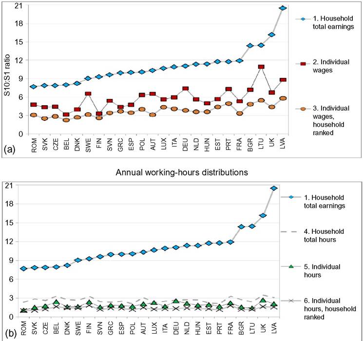
Figure 18.7 Top-to-bottom ratios (S10:S1) for employed individualsand their households, 26 European countries, 2010. (a) Annual earnings distributions. (b) Annual working-hours distributions. Reading note: In Romania average household total annual earnings in the 10th decile of such earnings are 8 times higher than in the 1st decile;annual earnings of individuals in the 10th decile of such earnings are 5 times higher than in the 1st decile if persons are individually ranked, and only 3 times if they are ranked according to their households total annual earnings. Explanatory note: The sample concerns households receiving their main income from earnings. The top-to-bottom ratio is between the average level of the tenth decile to the first decile. Source: Salverda and Haas (2014, Table 3.2).
technique of decomposition (see Fortin et al., 2011 for an overview). The results may depend on the choice.
In one of the first studies, Shorrocks (1983) using the American PSID over 1968-1977 concludes that “Dollar for dollar capital income and taxes have more distributional impact than earnings, which in turn exceeds the impact of transfer income” (which is defined to include retirement pensions and annuities).
Van Weeren and Van Praag (1983) use a special data set covering seven European countries (Belgium, Denmark, France, [West] Germany, Italy, the Netherlands, and the UK) in 1979 to decompose income inequality into subgroups. Interestingly, they look, inter alia, at the employment status of the head of household as well as the number of persons contributing to household income. At the time both characteristics make the largest contribution to inequality in Denmark, although employment makes the smallest contribution in the Netherlands and the number of earners in the UK.
Blackburn and Bloom (1987) draw a careful comparison ofthe family annual earnings distribution and the individual annual earnings distribution for the United States over the years 1967-1985. Usingvarious aggregate inequality measures they find that annual earnings inequality has hardly changed, although income inequality has. Descriptively splitting the distribution in five parts, the change seems largely concentrated in what they term the “upper class,” family with earnings over and above 225% of the median. From a time-series regression analysis they conclude that particularly the growth of nonprincipal earners in those households contributes to this growth. Blackburn and Bloom (1995) draw an international comparison at various points during the 1980s. For the United States, Canada, and Australia they find that income inequality increased among married-couple families and that the increases are closely associated with increases in the inequality of husbands’ earnings. Evidence of an increase in married-couple income inequality is found also for France and the United Kingdom, but not for Sweden or the Netherlands. In various countries, that increased inequality of family income is closely associated with an increased correlation between husbands’ and wives’ earnings. A more detailed examination in Canada and the United States suggests that this increase cannot be explained by an increase in the similarity of husbands’ and wives’ observable labor market characteristics in either country. Rather, it is explained partly by changes in the inter- spousal correlation between unobservable factors that influence labor market outcomes.
Karoly and Burtless (1995) follow Lerman and Yitzhaki (1984) in decomposing the evolution ofthe Gini coefficient of American distribution ofpersonal equivalized incomes between 1959 and 1989, basing themselves on census and CPS data. Theyfindlargelythe same results as Burtless (1999) does for his more recent period. A large part ofthe reduction in income inequality before 1969 is attributed to the decline in earnings inequality among male heads of families. After 1969 the same group is responsible for more than one-third of the increase in inequality. Since 1979, the improved earnings of women have increased inequality as they were concentrated in families with high incomes.
Cancian and Schoeni (1998) consider 10 countries using LIS data for the 1980s. They find that the labor-force participation of wives married to high-earning husbands increased more than for those married to middle-earning men.[127] At the same time, the mitigating effect of wives’ earnings actually increased slightly in all countries. In their view an unprecedented increase in the correlation of earnings between the partners would be needed to make the effect disequalizing.
Evelyn Lehrer (2000) finds from the US National Survey of Families and Households that between 1973 and 1992—1994 the equalizing influence of the wife’s contribution grew substantially stronger—partly due to a decrease in the dispersion of female earnings relative to that of male earnings. This seems to contrast with Karoly and Burtless (1995); however, her finding relates to married couples and their earnings only, not to the full personal income distribution.
Del Boca and Pasqua (2003) consider husbands and wives in Italy between 1977 and 1998 using regional differences and the absence of wives’ incomes as a counterfactual. The added worker effect is found in households especially in the North where there is more acceptance and more choice of working hours and more child care support available. Here the reduction in the dispersion of wives’ earnings seems to have offset increases in the dispersion of husbands’ earnings as well as the increased correlation in the earnings between the spouses between 1989 and 1998.
Johnson and Wilkins (2003), following DiNardo et al. (1996), studying Australian inequality over the period 1975—1999, find changes in the distribution of work across families—for example, an increase in both two-earner families and no-earner families—were the single-most important source of the increase in private-income inequality, with such changes on their own accounting for half the increase in inequality.
Daly and Valetta (2006), using CPS data for the United States and adopting partly the method of Burtless (1999), in combination with the decomposition technique proposed by DiNardo et al. (1996), find a more substantial contribution (50-80%) of men’s earnings to increased American inequality between 1969 and 1989 than does Burtless. This increase was counteracted by the growing employment participation of women. They explain the larger role of males as their methodology can account for growing inactivity and unemployment.
The Review of Economic Dynamics’ Special Issue of 2010[128] presents an interesting and important inventory of various dimensions of economic inequality, including the distributions on both sides of the individual earnings versus household incomes divide as well as the distributions of wages versus that of hours. The set of papers for seven countries contains useful descriptives of the distributions. In addition, some decomposition exercises are done on the log-variance of either earnings or hours. These decompositions concern a limited but important range of characteristics (gender, education, age, experience, region, family structure). They appear to explain little of the evolution and, in virtually all cases, leave most of the action to the residual. Of particular interest is Figure 18.8, where panel (a) specifies the variance of log individual hourly wages and panel (b) that of individual annual hours worked. The two are at different levels, the latter nowadays being much lower than the former, and their evolution seems to trend in opposite directions, clearly up for the former and declining for the latter. For annual earnings—seldom known from the contributions—the implication is a more substantial variance, which then feeds into household earnings.
Lu et al. (2011) study Canadian developments in the family earnings distribution (equivalized) from 1980 to 2005 using census data for those 2 years and 1995. They again adopt the decomposition approach developed by DiNardo et al. (1996). For 1980-1995 they find substantial increases in family earnings inequality, but for 1995-2005 some decrease. Changes in the earnings structure, such as those attributed to educational attainment, and changes in family composition (fewer married couples, more single individuals and lone parents) have been key factors contributing to growing family earnings inequality. Substantial changes in family characteristics (including a surprising decline in educational homogamy and the implied mating of women below their level) have had the most important counteracting effects as has continued growth in women’s employment rates. Interestingly, the authors take a special look at the Top 1% of the distribution, mention that it has increased substantially between 1995 and 2005 in contrast with declining family earnings inequality; however, they do not further highlight this in their analysis.
Larrimore (2013), again focusing on American CPS data, now for 1979-2007, and with the help of a shift-share decomposition, finds important differences between the three subsequent decades: changes in the correlation of spouses’ earnings accounted for income inequality growth in the 1980s but not in the 1990s (consistent with Figure 18.6). During the 2000s changes in the earnings of male household heads diminished income inequality, and the continued growth in income inequality was due to growing female earnings inequality and declining employment of both genders.
Finally, the most extensive decomposition study seems to be the one reported by Brewer et al. (2009) and Brewer and Wren-Lewis (2012). For the National Equality Panel (Hills et al., 2010) they have dissected the trends in British inequality over the long period 1968-2006 in many respects using a regression-based decomposition technique developed by Fields (2003) and Yun (2006). The results are presented in Figure 18.9. Total inequality of all households (line with white markers) moves to a higher level over the 1980s, from less than 100 to more than 160. The contribution that
18
Unfortunately they compare gross earnings to equivalised disposable household incomes, but they do decompose between (aggregate) taxes and benefits.
Log hourly earnings
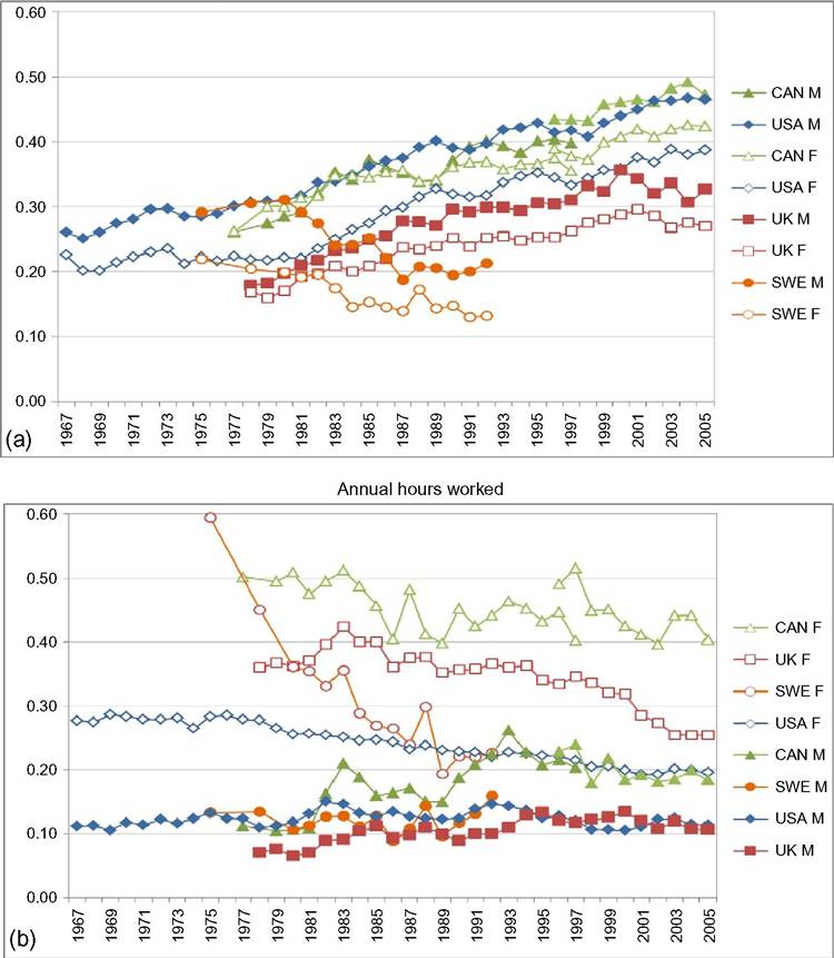
Figure 18.8 Evolution of variance, by gender, ages 25 to 59, United States, United Kingdom, Canada and Sweden, 2010. (a) Log hourly earnings. (b) Annual hours worked. Reading note: The variance of log hourly earnings of US males increased from 0.26 in 1967 to 0.47 in 2005. Explanatory note: F—females, M—males. Source: Blundell and Etheridge (2010), Brzozowski et al. (2010), Domeij and Floden (2010), and Heathcote et al. (2010).
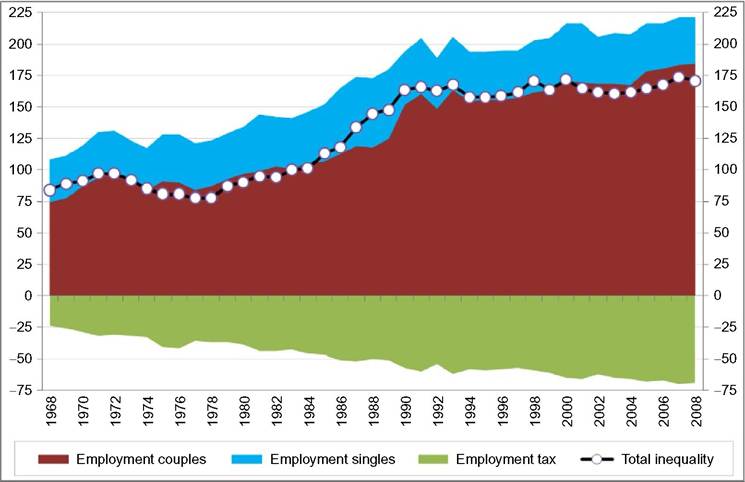
Figure 18.9 Contributions of household earnings to total net-equivalized household income inequality, United Kingdom, 1968-2008. Reading note: The line of total inequality results from adding up the contributions to inequality from couples and singles in employment and subtracting the tax they pay. Explanatory note: Inequalities are measured as the variance of logs (?1000). Contributions do not exactly add up as nonemployee categories receiving market income, pension have been left out. These contributions happen to partly cancel out but their aggregate has grown from 0 points in 1968 to 19 points out of the total of 171 that is shown for 2008. Source: Brewer and Wren-Lewis (2012, Table 5).
household gross earnings makes to this is split between the single-earner and dual-earner households respectively and the total of taxes paid by both (stacked shaded areas). The role of singles has remained unchanged on balance, with a temporary increase during the 1980s. Dual earners run largely parallel to total inequality; their growth is also somewhat concentrated to the 1980s though it continued after that at a slower pace. Taken together single and dual earners lag the inequality growth of the 1980s somewhat. That gap is filled by incomes from self-employment, investment, and pensions whose role more than doubled during the 1980s (not shown).[129] The net effect of earnings is less as taxation (the negative area which needs to be deducted) has also increased. After an initial rise up to the mid-1970s the rise is more gradual and extends over the period as a whole but hardly changes relative to earnings.
19
At the end of this overview a careful and detailed comparison of these results, including replication studies, seems advisable to find out where they diverge or even contradict and to seek an explanation whether differences are real—i.e., related to the period or the sample that is the focus—or artificial—i.e., due to the data set, the method of decomposition, or the approach to equivalization. Unfortunately, however useful, such a meta-analysis is entirely outside the scope of our contribution.
18.2.2.3 A Heuristic Help for the Role of Institutions and Earnings
Though we cannot and will not pursue a comprehensive approach to wage dispersion and income distribution, we may still ask what we can learn from the above and take with us for the contemplation of wage dispersion and institutions. We need to keep in mind, first and foremost, that labor market earnings make a major contribution to household incomes as well as their dispersion. By implication, the lack of such earnings resulting from unemployment or joblessness makes a large contribution, too.
Important developments are found that tend to diminish the direct influence of wage dispersion on the income distribution as the growing female labor market participation and at the same time enhance the role of household joint labor supply. This complicates the relationship between the two distributions, and it may also affect the labor market behavior of labor supply. Anyway, it brings into play a collection of new institutions that may affect both employment, hours worked, and pay, as well as their concentration across households. This may influence the level of wage inequality. It seems advisable to take the new institutions into account in addition to the traditional ones arising from labor market analysis on its own.
Another important inference to draw is the importance of considering hours and their dispersion in addition to wages. The inclusion of hours is important for several reasons. They are needed to arrive at the full picture of the earnings input that the labor market makes into household incomes. The hours dispersion differs significantly between the sexes, between countries, and also changes over time. In addition, the growing role of part-time and temporary jobs in itself makes this a more important dimension, and one that may also play a role in determining the dispersion of pay given the correlation between hours and pay. There may also be different trade-offs between hours and pay in different countries. At the same time, the role of hours may be relatively less important; it is more modest because of natural constraints than that of pay in an international comparison.
Second, it seems safe to conclude that one size does not fit all (countries). Significant differences are found, especially between different periods, and these seem to get more attention the further behind the period is (witness Larrimore’s most detailed account of such periodization in his 2013 publication).
Interestingly, comparable decompositions of important characteristics such as gender, age, education, and family type seem to play an amazingly small and also often flat role in virtually all countries, leaving a large role to residuals, which may point to national idiosyncrasies.
18.3.