WAGE DISPERSION: MEASUREMENT AND STYLIZED FACTS
Before we turn to the analysis of wage inequality and institutions in Section 18.4 we discuss here first the ways to measure these and then present what seem to be the current stylized facts of the literature concerning wage inequality.
Section 18.3.1 starts with a discussion of the issues involved in measuring wage inequality and a quick presentation of data sources. This is followed by a presentation of the “stylized facts,” which we define as the state-of-the-art knowledge of wage inequality currently accepted by scholars as necessitating explanation in spite of their different views and approaches. These facts regard, first, the aggregate level of inequality, referring to the most comprehensive distribution at the national level. For this we discuss outcomes according to different measures of inequality as well as for different definitions of the wage variable. Second, Section 18.3.2 considers disaggregate inequality, which highlights specific parts of the distribution—such as the tails or the middle—on the one hand, and inequalities among various subsamples of the population according to demographic or labor market criteria on the other hand. Then (in Section 18.3.3) we provide some new empirical evidence from a cross-section comparison of 30 countries for the most recent year available, which we elaborate on when our empirical approach in Section 18.3.4 concludes.18.3.1 Measuring Wage Inequality and Data Sources
Blackburn and Bloom (1987) have argued in detail the need of precision for measures and definitions of wage inequality. 0 Following their suggestions, we need to pay attention to at least four dimensions:
20 “The often-contradictory conclusions reached by studies of recent trends in income and earnings inequality are largely explained by the reliance of researchers on a remarkably wide range of conventions of data analysis.
For example, the list of important dimensions in which previous studies vary includes: the time period covered; the way family units are defined; the population to which the studies of individual earnings generalize (e.g., all earners, private nonagricultural workers, male earners, wage and salary workers, full-time, year-round workers, etc.); the measures of earnings and income (e.g., total family income, equivalent family income, total family earnings, wage and salary income, etc.); the unit of time for the measurement of earnings (e.g., annual, weekly, or hourly); the nature of the earnings measure (e.g., usual earnings or average earnings); measures of inequality (e.g., the Gini coefficient, income-class shares, variance of logarithms, coefficient of variation, mean logarithmic deviation, etc.); the use of individual or grouped income/earnings data; the treatment of sample weights; the treatment of observations with imputed incomes; the handling of top-coded values of income and earnings; and other criteria for including observations in the sample, such as the age of the respondent and whether the respondent was working at the time of the survey or in the year preceding the survey” Blackburn and Bloom (1987, 603).(1) the measure of inequality
(2) the definition of the wage variable (including its time dimension)
(3) the selection of the sample of the population that is being covered
(4) the nature of the data sources.
Clearly, the study of wage inequality adds several significant issues of measurement to those of long-term concern to the study of inequality (e.g., Atkinson, 1970; Chapter 5; Jenkins and Van Kerm, 2009). We consecutively address these four issues before we turn to data sources, and to the stylized facts in the following section.
Before starting this we mention a general observation. Wages are defined here as “wage rates,”[130] preferably controlled for hours worked[131] and therewith for differences in workers’ efforts, whereas we consider “earnings” or “wage earnings” as the product of those wage rates with the hours worked and therefore reflecting also differences in individual efforts.
For convenience we say in general that we are addressing “wage inequality.” However, this does not mean that we restrict ourselves to the inequality of wages rates only; to the contrary, we aim to also consider the dispersions of hours and earnings.When doing so we will try to be clear and not just mention wages but use the appropriate concepts: weekly, monthly, or annual hours or earnings.[132] Wage rates serve the clear analytical purpose of enabling comparisons between individuals on the basis of the same efforts made in terms of time dedicated to paid work, measured in hours. As already argued, hours are an increasingly important dimension of labor market functioning and inequality and will be given their due.18.3.1.1 MeasuresofInequality
Although the Gini coefficient is a very popular measure in the analysis of income inequality, it hardly figures in the analysis of wage inequality. Variance, mean log deviation, the Theil index, and standard deviation are used, however.[133] Unfortunately, because of their aggregate nature, these measures tell us little about where in the distribution the differences over time or across countries reside, though decomposition of these measures, as far as possible, can certainly be helpful for understanding the underlying processes. In wageinequality analysis it is the percentile ratios that play a remarkably important role: the P90: P10, P90:P50, and P50:P10 ratios, which mutually relate the 10th, 50th, and 90th percentiles to each other.[134] These ratios are directly helpful in focusing attention on particular parts of the wage distribution and they are intuitive at the same time. Their evolution over time reflects differential changes in wages at specific points of the distribution. As we will see below, up to this very day the debate on the effects of the minimum wage on wage inequality is framed almost exclusively in terms of these ratios. The ratios have also provided important leverage to the shift that has occurred in the debate about the role of technology as a determinant of growing wage inequality.
Their popularity may relate also to an easier consistency with the analytical focus on the individual and his or her efforts in the labor market in contrast to income analysis.[135] Note that the ratios are based on the upper-boundary wage levels of the chosen percentiles (or deciles), andnot on their means, sums, or shares in the total of wages. This implies certain limitations to the use of these ratios, and it seems advisable to add measures that broaden to averages, sums, or shares. For example, a top-to-bottom ratio between the means, sums, or shares of the top decile on the one hand and that of the bottom decile on the other hand (denoted as S10:S1) may find inequality growing much farther apart than the P90:P10 ratio would suggest, if important changes are actually occurring within the two tail deciles and affecting their within-spread.[136] Precisely that is the upshot of the recent analysis of top-income shares, where the sum and the share of the top decile, and its within-distribution over smaller fractions, are the very subject of study. In a similar vein, much of the current minimum-wage debate appears to be effectively analyzing changes found within (and perhaps even restricted to) the bottom decile of the wage distribution. Note that the OECD has recently introduced the top-to-bottom ratio in its income inequality and poverty database.[137] [138] In addition to these quantile ratios, the ratio between the average wage and the median wage is sometimes also found as an indicator of wage inequality; the Kaitz index similarly relates the level of the minimum wage to the average wage in the analysis of minimum wage effects. One disadvantage of all such ratios, however, is that they cannot be decomposed (Lemieux, 2008, 23), 9 though they may be further split into ever smaller fractions.Some other indicators are available in the same family of disaggregate measures that can also relay information about wage inequality.
These relate to parts of the distribution that are defined with the help of an external wage-level criterion. The most important one in practice, regularly published by the OECD, is the incidence of low-wage employment (see Gautie and Schmitt, 2010; Lucifora and Salverda, 2009). This is defined as the share of all employees in the wage distribution who are found having wages below the level of two-thirds of the median wage.[139] It is important to realize that this is a concept that relates to the analysis of the labor market, in contrast with in-work poverty that depends on the household-income position of the wage earners concerned; nonetheless the former is definitely relevant to the analysis of the latter. The concept of low pay is only infrequently used in US analyses of wage inequality where the in-work poverty concept is more frequent, perhaps because the poverty threshold is of such central concern in that country’s public discourse.[140] The divergence between the two concepts signifies that workers may be poor—on the basis of their household situation—at wage levels that are well above the low-pay threshold, and vice versa, that workers receiving low pay may be found in households well above the poverty level.[141] Unsurprisingly, the evolution over time may differ between low pay and poverty wages. Figure 18.10 clearly points this out for the United States. Overthe period 1995—2002 the share of employees earning poverty wages shows a particularly sharp decline, although the incidence of low pay remains unchanged. Household composition, household joint labor supply, and the evolution of prices determining the poverty lines can influence the former but not the latter, which depends on wage developments.As an analogue to low-wage employment one can conceive of the incidence of pay at or below the minimum wage as another simple measure of wage inequality. Strikingly, in spite of decades of intense debate on the employment effects of the minimum wage such
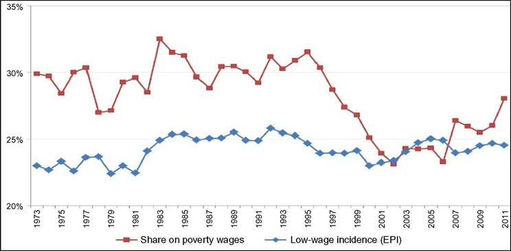
Figure 18.10 Shares (%) of workers earning a poverty wage or a low wage, United States, 1973-2011.
Reading note: The percentage of all employees earning a poverty wage fluctuates around 30 until 1996 and then falls substantially;the percentage earning a low wage fluctuates around 25 from 1983 onward. Explanatory note: Poverty wages are earned by individuals whose household incomes are below the official poverty threshold;low wages are defined as being at or below two-thirds of the median wage: on authors' estimation for hourly earnings of all workers using linear interpolation in the decile distribution. Source: Authors' calculation on EPI, State of Working America 2012, data underlying Figure 4E and C.statistical data are sporadic. Internationally, a possible explanation may be the nonuniversality of statutory minimum wages or their complex nature when, for example, it is less evident to whom they apply or not—a problem that is absent in measuring the low pay incidence.
Finally, as implictly suggested above, the share of top wages in the wage distribution—a direct corrollary to top-income shares—provides another possible statistic that can throw light on wage inequality. We will see later that pay at the top plays an increasingly important role in the wage-inequality debate.
18.3.1.2 Definitions of the Wage Variable[142]
Most of the literature restricts the definition of the wage variable to the payments received by employees from their employers, and we will follow that convention here. This excludes for reasons of principle both the unemployed and the self-employed (however, this does not mean that they should be excluded from the analysis of labor markets and wage inequality—compare our approach in Section 18.5). We will focus on gross wages, including taxes and contributions, which are paid by the employee (also when the employer actually withholds them on behalf of the tax authorities). However, gross wages are not available for all countries all of the time though, fortunately, they now increasingly are (e.g., very recently France, Greece, and Switzerland started to provide gross wages; net wages will likely show a lower level of inequality because of tax progression). In addition, even gross wages are a more restricted concept than “employee compensation” in the sense that they exclude employer contributions such as for occupational pensions and other provisions. This is for the practical reason of lacking observations in most countries.[143] The full-gross wage defined as employee compensation including employee taxes and contributions seems the most appropriate concept in principle as it includes what can be called the “social wage.” This encompasses entitlements financed out of employee and employer contributions and income tax, and varies significantly between countries (Gautie and Schmitt, 2010). Finally, the wage concept mostly comprises payments that are actually made by the employer and may leave out informal cash payments such as tips, in spite of their (suggested but often statistically unknown) importance for low-wage earners in some countries.
Given this definition of wages, there is one crucial dimension about which we aim to be as clear as possible. This regards their time dimension, which appears to greatly influence the apparent level ofinequality. We have already touched on this above when mentioning the distinction between hourly wage rates and their multiplication by hours worked. Most of the US inequality debate has been framed in terms of full-time weekly wages if not fulltime full-year wages (Acemoglu and Autor, 2011, 1049)—“earnings” in our definition. Though this seems largely a matter of data convenience, it may have important implications for comparisons. First, it ignores the incidence ofpart-time employment which varies significantly overtime and across countries. Second, it overlooks the dispersion of full-time working hours itself, which can be considerable and may differ between countries.[144]
Third, different time periods for wages/earnings bring into play different, additional elements of pay such as bonuses and other special payments that are made with a lower frequency, for example, on an annual basis. Such payments usually have an increasing effect on inequality, which risks to be missed by a shorter time horizon—the use of an annual average of shorter-term wages can potentially mend this problem, but this is not standard practice.
Fourth, the use of time for the weighting of the observations bears on the level of inequality, too. This issue regards the working hours of the employee. Pay observations—including for hourly pay—can be taken simply over the head count of employees or alternatively over the count of hours worked, that is over employees weighted by their working hours. The latter boils down to full-time equivalent wage levels and lends part-time employees a lesser weight in determining the average and the quantiles. Evidently, such weighting reflects more closely the economics of the labor market and less the receiving side of labor’s personal incomes, which affect their significance for household welfare and spending; both sides deserve consideration, and attention should not focus exclusively on one or the other.
Finally, there is yet another timing issue on the employee side: wages can concern all who are in work during a year or they may be restricted to those who work the full year, or alternatively all workers may be considered in terms of full-year equivalents. Covering all includes the people who enter or leave employment (or both) in the course of the year; in the full-year option they are left out, in the annualized full-year equivalent approach they will be weighted also by the part of the year in which they work. The share of part-year workers naturally differs between social groups, but it can differ also over countries and over time, because of the business cycle or because of a different or changing role of temporary jobs. New entrants in particular may have low wages and significantly affect inequality at the left-hand tail of the distribution. Finally, the part of the year they actually cover—say 3 months instead of four—will affect their earnings considerably and may have a significant effect at the margin on annual earnings inequality.[145]
To conclude, we do not think there is one best definition of the wage or earnings variable—it depends on the purpose of the analysis. We do think that definition and purpose should be explicit and mutually consistent and that shortcuts adopted for reasons of data covenience should be scrutinized for their hidden properties and potential effects on the outcomes.
18.3.1.3 Composition and Samples of the Population
Another issue worth mentioning is the part of the population that is covered by the analysis. A pars pro toto approach, that views a part ofthe population as representative ofthe whole, is particularly dangerous in inequality analysis. Subsets of the population may occupy very different positions in the overall distribution, and inequality may differ significantly between them. Their inclusion or exclusion can exert large marginal effects on the level of inequality even when they are relatively small compared to the whole population. Selection along dimensions such as gender, age, education, or experience on the side of the person, or industry, occupation, the nature of the employment contract and its protection, and the (part-time) working hours on the side of the job can greatly affect the aggregate outcome. The issue may seem obvious although it frequently is a source of error, confusion, or even distortion. For example, contributions may focus on men, on people working full time, on the working-age population, or on positive incomes only, as if assuming that all the rest of the population makes no difference to the general outcome nor to that of the selected group. Imagine that women increasingly occupy low-paid jobs while men are ousted and leave employment; both groups could potentially see their wage inequality fall, though overall it might actually increase. Another realistic example is from Krueger and Perri (2006), who draw conclusions about household consumption inequality for the United States as a whole on a (laudably specified) sample that leaves out non-workingage households, those without an income from labor, and rural households—which are groups that may substantially affect inequality at the margin. Finally, even if all the population is covered all the time, compositional shifts across categories may be highly relevant to the evolution of inequality and will need proper scrutiny. Vice versa, aggregate stability of inequality can go together with changes in inequality within many distinct categories; in the extreme case, even all categories could face inequality change in the same direction (together with shifts in their positions relative to each other). Finally, it is important to add the observation—found in the overview of the literature below—that the distinction of between-inequality and within-inequality (the residuals, after all) depends on the variables chosen as the basis for the decomposition. That choice will likely be inspired by what are considered to be the stylized facts; as a consequence, insufficient attention may be paid to the implications of large residuals and these may actually obtain an importance of their own as is underlined by some of the literature that we will be discussing.
18.3.1.4 Data Sources/Statistical Observation
Individual wages seem more cumbersome to observe statistically than household incomes. For incomes, the collection of taxes provides a strong and universal incentive for gathering administrative data. Such data usually combine considerable precision regarding the core variables with clear limitations for other variables such as personal characteristics, for example, educational attainment is of no direct importance to the tax authorities. This motivation may be less compelling for a comprehensive collection of wage data. Administrative data may be gathered for registering individual Social Security entitlements, but their nature and coverage will depend on the idiosyncracies of the entitlement rules; for example, the sampling may be restricted to those who can qualify for the entitlements in question (e.g., after a probation period, working a minimum of hours, excluding overtime earnings), or focus on their work histories and not their actual earnings, or cover their earnings up to a relevant threshold only. This may hamper their use particularly in international comparisons.
Dedicated surveys, by contrast, require a special effort and consequently are subject from the start to cost-benefit trade-offs, which will affect the range of variables, the population samples, and the time periods covered. This explains why surveys may concentrate on information that is easier to collect, and also that significant international differences occur in the availiability of data and in their coverage. As a result, one can understand the long-time focus in OECD data and American data, along with analyses of full-time workers : collecting hours information on top of earnings information to enable determining hourly wages, or information on workers who have left during the year on top of those permanently employed or present at the time of the survey, is simply more demanding and costly. This may be the case particularly if the information is gathered from employers. Note, though, that ICT developments are greatly facilitating the transfer of firm data to statistical offices. Employers will, by their own interest, dispose of the most accurate information about pay. By contrast, if the information is gathered from households, the information on wages will be less precise, as respondents may not know the details of wage components or taxation and contributions, or respondents may actually be less well-informed than other members of the household. Equally, the information about hours of work may differ between employer sources and household sources, as the former will focus on legally formalized working time whereas the interest of the latter will be in the actual hours that a job involves, possibly including the necessary travel times. Interestingly, a concentration on full-time full-year workers may make little sense in a household survey as it will add to the costs. At the same time, employers will be less well informed about workers’ personal characteristics such as educational attainment or the worker’s household situation, and the availability and quality of that information from a household survey may be superior compared to employer surveys. Another advantage of administrative tax data can be their more comprehensive time coverage—tax is paid over the full year—whereas household surveys may have important
37
Stretching all the way from the 1980s to Acemoglu and Autor (2011) included. Heathcote et al. (2010, 24) point out the inadequacy of this focus.
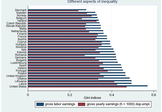
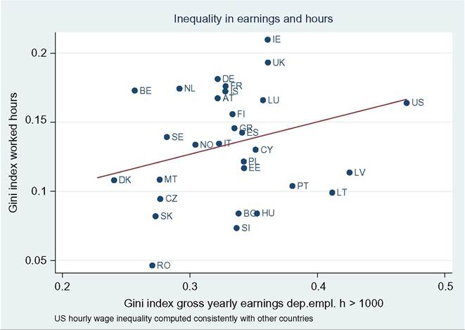
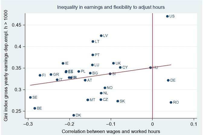
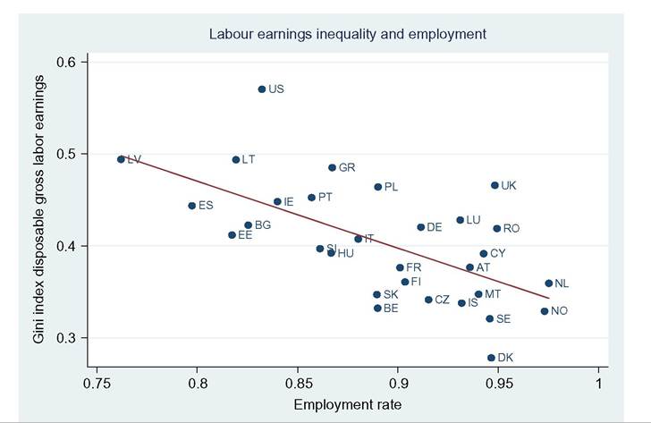
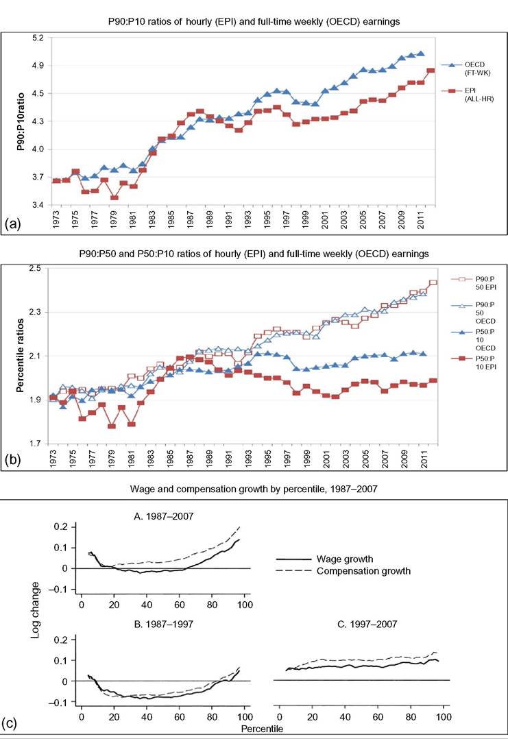
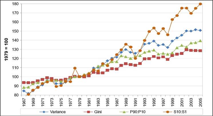
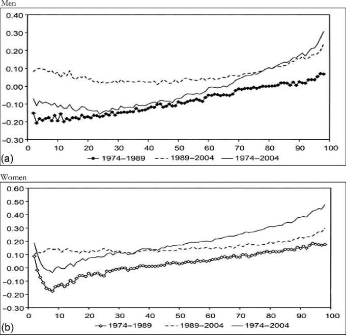
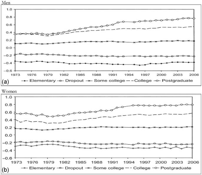
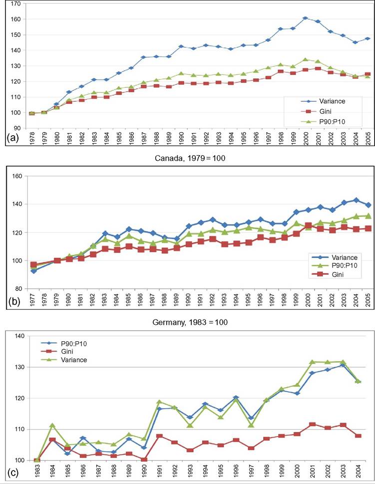
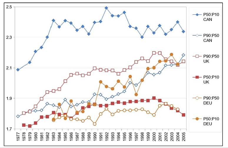
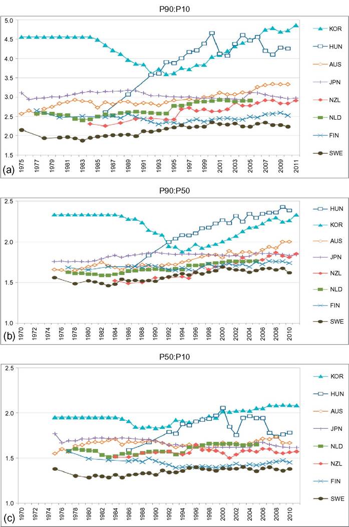
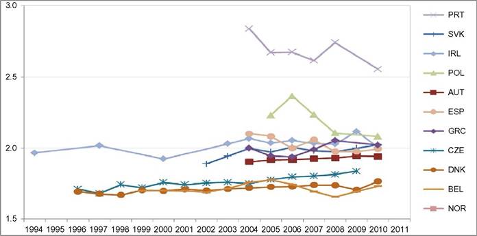
limitations, such as what time of the year the survey questions are asked—do the questions relate to the preceding year or the current one? Adding the dimension of hours to that of earnings can only complicate this.[146] Finally, administrative data will normally cover very large shares of the population and ascertain that all essential questions are answered, whereas other surveys can cover only much smaller samples and suffer from considerable nonresponse to questions,[147] [148] generating less-accurate results also as a consequence of that. Nonresponse will be more important for the current focus on wages at the very top; unsurprisingly, tax data play a large role here though the top-coding of responses may still affect the availability of data, but that is no different for wages than for incomes. As administrative data will be available anyway, increasingly, the statistical offices are trying to use these instead of asking fresh questions to households or firms, and use those data for imputations in other surveys, blurring the distinction between the two types of information as a result. Naturally, both administrative and survey data are subject to changes over time. The tax system or Social Security rules may change and ask for new variables or drop existing ones. A survey may be adapted also because of costs, or simply because a new survey is started without paying due attention to the continuity with its precedessors.40 Having said this, the main data source in the literature is first and foremost the American Current Population Survey CPS. It is a household survey, started in the 1940s and providing tabulated data from then, that has made microdata available for research since the early 1960s (the more adequate CPS ORG—outgoing rotation groups—data being available since 1979 only). CPS comes in different “tastes”: the March CPS or the May and/or ORG CPS, and one needs to be careful which one to use, partly depending on the purpose of its use. The March CPS is not good for hourly wages, whereas the CPS ORG does a better job here and also has a much larger sample size than the May CPS, which, in addition, may be seasonally affected while the ORG CPS data cover the full (preceding) year.[149] However, the practice of top-coding of labor incomes may reduce the usefulness of this source of data for studying earnings inequality.[150] Several other American data sources are sometimes used, such as the PSID (which we will use below for better mimicking European SILC data) and the census, and also employer surveys such as the Employment Cost Index microdata (Pierce, 2001, 2010). Second, on the EU side, increasingly two consecutive EU-wide (panel) surveys provide microdata for research: the European Community Household Survey (ECHP) and the Statistics on Income and Living Conditions EU-SILC. The ECHP covers the EU15 only, with the exception of the first years of Austria, Finland, and Sweden, who joined the EU in 1995. The survey performed eight annual waves in the years 1994—2001, generating annual data for the years 1993-2000. Sample sizes and degrees of panel attrition diverge substantially across countries depending on the value attached to the survey in the country.[151] The ECHP was discontinued and has been replaced with EU-SILC, which is still in force today. SILC has annual waves starting in 2003/2004 and extending to 2012 at the time of writing—again relaying full-year data for the preceding years (in most countries). SILC’s country coverage follows the extension of EU membership and attains full coverage ofEU-27 together with Iceland, Norway, Switzerland, and Turkey in 2007.[152] There are a host of small differences between countries in sampling, definitions, and the like, and these also change over the years. Importantly, the gross wage variable has been available for all countries since the wave of 2011, although up to then some countries provided net wages only (France, Italy, Switzerland).[153] Another easily accessible and often-used international data set is the OECD’s earnings database, which provides tabulated data. It has been built since the mid-1990s and now covers 34 countries,[154] albeit with rather uneven time coverage. Only seven countries go back in time before 1990, and complete coverage is very recent (2010). In most cases the data are provided by the national statistical offices, although in a few cases they are derived by the OECD from other surveys or provided by national experts. However, definitions and samples vary widely between countries, covering the entire set of possible differences that we have just discussed, ranging from all all individual employees to full-time, fulltime full-year employees, and full-time equivalent employees, from hourly wages to weekly, monthly, and full-time equivalent annual earnings, and from gross to net after taxes and contributions. The latest version of the full database contains 90 different series endorsing 33 different definitions. It commonly details the outcomes also for the two genders. For the website version of the database, the OECD has chosen to present only one series per country, 33 in total. This reduces diversity to nine different definitions; the mode (20 series) concerns full-time employees’ weekly or monthly gross earnings (which may be deemed reasonably comparable[155]) but only 11 of those go back in time before the year 2000. All definitory properties are admirably documented in the database and offer the user the opportunity to consider the differences and their potential effects. Nevertheless, the database is clearly not immune to the problems of secondary data sets that Atkinson and Brandolini (2001) have stressed for incomes, but which are equally important for wages and earnings.[156] Finally, Atkinson (2008) provides the results of an in-depth study of the earnings distribution in 20 countries, inspired by the work of Harold Lydall (1968). He advocates a long-run picture on a year-by-year basis, showing that “drawing on isolated years... can be misleading.” For each country an extensive appendix documents the available data sources and the properties of the data and the presents the evolution at various percentiles of the distribution, ranged separately for the lower and the upper half of the distribution. The series end in 2004 and stretch back in time to well before those of the OECD database. For 15 countries they start before 1960 and cover most of the postwar period and some of those (Canada, France, Germany, United States) go back to before the war.[157] This long time span helps to realize the particular nature of the more recent developments that are the subject of the debates considered in this chapter. Roughly speaking, strong declines in inequality over previous decades preceded the increase on which the literature started to focus in the 1980s. Preferably, the analysis should be able to also explain the declines. To conclude it seems natural that contributors to the literature are requested to specify their definitions, samples—including censoring or top-coding—as well as sources. Given the long history of using the CPS this is increasingly becoming standard practice in American contributions, but it certainly needs endorsement in international comparisons. Equally important, but not frequently practised, it seems highly advisable to consider the possible implications that data limitations and data choices made may have for the conclusions that are drawn. 18.3.2 Cross-Country Levels and Evolution ofWage Inequality We now turn to the stylized facts of earnings inequality as we derive them from the literature. This is done in two steps. We start with the United States, which is the country having the best information and where the debate and the analysis of earnings inequality have developed most strongly, enabling us to spell out most of the issues at stake. We contemplate the variation in outcomes between different measures of inequality where feasible, between different definitions of the wage variable where necessary, and between different data sources where reasonably available. In addition to discussing aggregate outcomes, we take a look at some breakdowns—both of the earnings distribution itself and by segments of the (employee) population. Next to the United States, we continue with a consideration of various other countries aimed at comparing the inequality trends but also at identifying gaps in the available data that hamper comparability. In Section 18.3.3 we provide some new empirical evidence from a cross-section comparison of the EU countries and the United States for the most recent year available, based on EU-SILC and PSID, which we will use for our empirical approach in Section 18.5. We end with summary conclusions regarding the stylized facts in international comparison. 18.3.2.1 U.S. Earnings Inequality Much of the American literature focuses on men or at least distinguishes between the sexes, treating them separately and seldom putting them together in the overarching distribution. This contrasts with other countries and seems a paradox as US female employment started growing earlier than elsewhere and also grew more fiercely in the sense of being predominantly full time and extending high up the overall earnings distribution (Salverda et al., 2001). It may be explained from the early start of the inequality debate in the United States at a time that data did not really allow putting them together. This split risks ignoring the genders’ mutual interaction in labor supply and demand and overlooking also the contribution of the within-country doubling of the labor force between the late 1960 and mid-2000s, which has remained in the shadow of the worldwide Great Doubling, a term famously coined by Freeman (2006). For this reason and for the sake of international comparability, and also because it allows covering the recent years since the mid-2000s, we start with a quick look at the aggregate level of all employees irrespective of gender. That comprehensive picture is provided by Figure 18.11. Panel A indicates the overall percentile ratio, P90:P10, from two different sources, the EPI’s State of Working America and the OECD’s Gross Earnings Database. EPI covers hourly wages of all employees, presumably based on head count individuals and not full-time equivalents; the OECD data, by contrast, concern weekly earnings of full-time employees and therefore miss out on part-time employment. Starting at exactly the same level in 1973, EPI shows a much stronger increase in the ratio between 1979 and 1988 than OECD, directly followed by a decline while the OECD series remains unchanged. At the end the inequality level according to EPI is well below the OECD’s.[158] [159] The conceptual difference between the two is important as it is found throughout the literature. Lemieux (2010) as well as Heathcote et al. (2010) provide state-of-the-art overviews of developments for many aspects of American earnings inequality from around 1970 to the mid-2000s, entirely based on hourly wages (but always split by gender). Other important contributions (e.g., Acemoglu and Autor, 2011), by contrast, draw to an important extent on full-time weekly or full-time full-year workers (equally split by gender). Autor et al. (2008, Figures 2 and 3) draw a useful comparison between hourly and full-time full-year earnings inequality trends. Panel (b) pictures the percentile ratios of the common split between the upper and the lower half of the distribution from the same two sources. It suggests that the difference between the sources and the definitions concentrates in the bottom half; in the upper half the two series are almost identical, which is understandable as in this case virtually all employees will be working full time. The divergence between the two halves is an important observation to retain. The panel also suggests, in accordance with much of the literature using the gender breakdown, that developments since the early 1990s have been different from before, because, on the one hand, lower-half inequality hardly changes in contrast to the preceding period, but upper-half inequality keeps on growing relentlessly, with ends far exceeding bottom-half inequality. With the EPI data, the divergence starts in 1992, with the OECD in 1995. Finally, panel (c) adds a rather different way of presenting the evolution ofinequality: the cumulative changes in real wage levels for each of the 100 percentiles over different time periods, using the work by Pierce (2010). This has become a convenient way of presenting the data in the polarization debate that we will report on later. The discontinuous periodization highlights apparent differences but may suffer from a certain arbitrariness at the same time. With its detail, this type of presentation seems to implicitly Figure 18.11 Inequalityofindividual earnings, United States, 1973-2012. (a) P90:P10 ratios of hourly (EPI) and full-time weekly (OECD) earnings. (b) P90:P50 and P50:P10 ratios of hourly (EPI) and full-time weekly (OECD) earnings. (c) Wage and compensation growth by percentile, 1987-2007. Sources: OECD Gross earnings: Decile ratios (26 October 2013), Economic Policy Institute EPI, State of Working America 2012, Washington: Real wage deciles, all workers, 2012 dollars (based on data from the CPS), and Pierce (2010, Figure 2.5) (based on Employment Cost Index data). Figure 18.12 Four measures of hourly wage inequality: United States, Men only, 1967-2005, 1979 = 100. Reading note: S10:S1 is the ratio between average hourly wages in the top decile to the bottom decile. Explanatory note: Figures cover individuals aged 25-60 who work at least 260 h per year, with wages at least half of the legal federal minimum wage. Source: Heathcote et al. (2010, Figure 4) and S10:S1 derived from Figure 7 (based on March CPS). criticize the use of more aggregated measures such as the Gini coefficient or the overall percentile ratio. The panel shows a much flatter pattern of changes over the 1990s than over the 1980s, when strong declines in real wages occur for most percentiles between the tails of the distribution. Nevertheless, real wage growth mostly increases with the wage level. Interestingly, the panel elaborates also on total compensation (dashed lines), which includes employer contributions on top of wages. This is a unique feature that will be mentioned only here. We may conclude from it that the comprehensive concept of earnings does not change the general patterns for the 1980s and 1990s though it reinforces inequality levels somewhat during both periods.[160] Figure 18.12 draws a comparison (for men only) of the intuitive overall percentile ratio with the often-used aggregate measures of log wage variation and the Gini coefficient and also with the ratio of average wages in the top and bottom decile (S10:S1). All measures show much higher levels now than in the 1970s. However, the variance grows substantially more strongly than the Gini coefficient, while the percentile ratio fluctuates between them, the S10:S1 ratio runs away from the rest after 19 93.[161] The divergence between the S10:S1 ratio and the common P90:P10 ratio implies that the rapid rise has to do with the within distribution of the two tails, which none of the other three measures seem to be able to capture adequately. The top-incomes literature has already shown its importance at the top end, but the dispersion within the bottom decile merits equal attention.[162] Apparently, the strength of the increase in the dispersion depends on the measure chosen and also their periodic ups and downs do not fully coincide. The top and bottom half split of Figure 18.11 has provided a first breakdown of the aggregate by focusing on parts of the distribution. The incidence of low pay or high pay, and the size of the remaining middle are indicators of the same sort. The former was already shown in Figure 18.10. It moves up from 23% in 1975 to 25% in the mid- 1980s and has been rather stable at about that level since. Over the same period the share of those high-paid, defined as earnings exceeding 1.5 times the median hourly wage, increases from 21% to 25% in the mid-1980s and further to 28% (not shown). As a result the remainder in the middle shows a considerable fall before the mid-1980s (55—50%) and another slighter fall over the current crisis (49—47%). A narrower definition of high pay following the top-incomes literature is pursued by Lemieux (2010), who endorses a simple repair for the top-coding of earnings in the CPS[163] and presents percentiles distributions similar to those of Pierce above, which we reproduce in Figure 18.13. Starting in 1974 the period covered is significantly longer but still split into two parts, now on both sides of the year 1980. Separate distributions are given for men and women. Again developments are more positive and spread more evenly over most of the distribution during the second period after 1989 than before. The longer period covered up to 1989 shows a more skewed picture than Pierce’s. Particularly, real wage change in the bottom 20% seems more negative now for men, although an increase in the lowest percentiles for women may help explain the surprisingly upward move found by Pierce. At the same time, it is clear that among men the high part of the distribution has run away from the rest with a steep gradient within the top decile. The top percentile ratios seem to support this (not shown). They are almost identical and trend upward together until the end of the 1990s when female inequality starts to lag behind. The bottom-half ratios run largely parallel to each other with the one for females indicating a substantially lower level of inequality. The more positive development of wages for women seem suggestive of a declining gender gap. This is borne out clearly by Heathcote et al. (2010, Figure 5) who, after a slight increase of the gap from 1967 to 1978, find a continuous decline after Figure 18.13 Percentage change in real hourly wages, by gender and percentiles, United States, 1974-2004. (a) Men and (b) women. Source: Lemieux (2010, Figure 1.7). that year, sharply up to the mid-1990s and more modest since then. The current gap (30%) is much smaller than before but certainly not negligible. Next to gender, educational attainment is the most important dimension for breaking down inequality. Its role has been a bone of contention in the literature from the start, as we will see later. Here Lemieux (2010) presents differentials for various levels of attainment relative to high school graduates (Figure 18.14). They appear to be mostly flat with slight declines at the lower levels but with the clear exception of the highest two levels, particularly the highest. These start growing away upward particularly over the 1980s and more modestly since. For men the top-bottom gap almost doubles. At the end of the period the differentials seem almost identical between the two sexes. Heathcote et al. (2010, Figure 5) present a college wage premium defined as the ratio between the average Figure 18.14 Educational differentials relative to the high-school level, by gender, United States, 1973-2006. (a) Men and (b) women. Explanatory note: Using a decomposition based solely on education and experience. Source: Lemieux (2010), Figure 1.3. hourly wage of workers with at least 16 years of schooling, and the average wage of workers with fewer than 16 years of schooling. The premium increases significantly though more for men (52—92%) than for women (58—69%). We stop here and refer for further detail of other dimensions of the earnings dispersion, such as experience or nationality/country of birth, to the literature itself.Before we continue we will stress again the important role of residuals. These outcomes for gender and education rest on simple decompositions, and most of the action appears to reside in the residuals, which develop largely in parallel to the growth in overall “raw” inequality (Heathcote et al., 2010, Figure 5). The implication is that other factors of influence need to be incorporated in the analysis and/or that idiosyncrasies, which may be immune to further analysis, play a nonnegligible role. Lemieux (2010, Figure 1.8) finds, interestingly, that the importance of residuals grows with the level of earnings, especially over the period 1974-1989. 18.3.2.2 Earnings Inequality in Other Countries We now turn to inequality trends in other countries. The Review of Economic Dynamics (RED) (2010) is a special issue dedicated to cross-sectional facts regarding elements of economic inequality; it provides the most precise cross-country comparison of the earnings dispersion and several of its important facets, using as uniform a template of data treatment and presentation as possible.[164] Unfortunately, it has several drawbacks. The limited number of countries of relevance here is only seven, and for our comparison it is even further reduced as Italy and Spain focus on earnings net after taxes, which are unsuited for a comparison to gross earnings, and relevant data for Sweden end in 1992 when the country’s financial crisis had just started. That leaves us with the United Kingdom, Canada, and Germany. We turn to these results first, and after that we turn to the OECD’s earnings database to see what we can learn for other countries. Figure 18.15 presents three measures of individual hourly earnings dispersion, for men and women together, as found in the RED contributions: the variance oflog wages, Gini coefficient, and overall percentile ratio. All indicators for the three countries tend to rise over time. The British variance increases very rapidly up to a level 60% above the start of 1978, which well exceeds the other two measures (and also the variance in the United States), and subsequently falls over the 2000s. The other two measures for the United Kingdom also show a decline over that last period. This contrasts with the OECD’s percentile ratio (not shown), which (covering full-time weekly earnings) is at a somewhat lower level but continues rising until 2006 and remains unchanged until 2011. For Canada the rise is also considerable, +20-40% depending on the measure, and continues until the end of the period. Mutual differences between the measures are smaller. The OECD’s percentile ratio (not shown), again for full-time weekly earnings and available after the mid-1990s only, shows continued growth over the entire 2000s. Finally, in Germany, data are available from 1983, the rise of the three indicators concentrates in the period after unification. The variance shows a clear rise, and it is virtually identical for the percentile ratio—in contrast with the other two countries. Taken over the same 1983-2004 period, their growth is stronger than in the United Kingdom or Canada. The rise of the percentile ratio must rest on the use of hourly earnings as the trend of the OECD’s ratio (not shown), which concerns full-time monthly earnings, is largely flat over the 1990s and early 2000s. However, the increase in the Gini coefficient is modest relative to the other indicators as well as the other countries. United Kingdom, 1979 = 100 Figure 18.15 Dispersion of hourly wages, United Kingdom, Canada and Germany, late-1970s to mid- 2000s. (a) United Kingdom, 1979 = 100. (b) Canada, 1979 = 100. (c) Germany, 1983 = 100. Explanatory note: Figures cover individuals aged 25-60. Derived from the data underlying Figures 3.1 (UK), 4 (Canada) and 6 (Germany) as posted on the RED website. Data sets concern for Canada the Survey of Consumer Finances SCF 1977-1997 and Survey of Labor and Income Dynamics SLID 1996-2005, for Germany the German Socioeconomic Panel GOEP, and for the UK the Family Expenditure Survey FES and Labor Force Survey LFS. Sources: Brzozowski et al. (2010), Fuchs-SchOndeln et al. (2010), and Blundell and Etheridge (2010). Figure 18.16 Lower and upper half inequalities in Canada, Germany, and United Kingdom, 1977-2005. Sources: Blundell and Etheridge (2010), Brzozowski et al. (2010), and Fuchs-Schundeln etal. (2010). In Figure 18.16 we split the overall percentile ratio into its two contributing halves, P90:P50 and P50:P10. We a find strong divergence between the countries. The high levels and strong rise of the bottom-half ratios in Canada and Germany[165] are strikingly different from the United Kingdom; the German ratio moves up as much as the British but over a considerably shorter period. Canada and the United Kingdom share a decline in recent years though. Upper-half inequality rises very little in Germany and clearly less than in Canada and the United Kingdom. Generally, the pattern of the two British trends is very similar to the United States in Figure 18.11, whereas Canadian trends look surprisingly different. This clearly call for further scrutiny.[166] Unfortunately, wage changes by percentile, which have come to play an important role in the American debate, are not available for other countries. The RED papers have also looked at the roles of gender and educational attainment. The gender pay gap for Canada is small from the start, comparable to the US gap at the end of the period (30%), and it trends downward only very slowly. The German gap declines slightly more steeply and ends below (20%) the American level in the mid-2000s. The British gap, finally, declines somewhat more strongly; it is below the US level in the late 1970s but ends at about the same level. Note again that the decompositions made in the RED papers are based on gender, educational attainment, and experiences only and that in these three counties, as in the United States, residuals are quantitatively important and behind most of the increase in inequality. With the help ofthe OECD’s earnings database of percentile ratios, the evolution of individual earnings inequality can be described for a number of other countries (see Figure 18.17). 9 As already stated it is a secondary database, and it has to be used with great care. It comprises a wide array of wage definitions and concomitant samples of the employee population. We first select eight countries that focus on gross earnings of full-time workers (be it hourly, weekly, monthly, or annually ) and also have a long-run series. Given the diverging incidence of part-time employment, the full-time focus will be more or less representative of the country, but there is nothing we can do about that apart from being aware that in (various European) countries where part-time jobs have become more important and tend to be overrepresented in the low-wage segment of employment, the actual picture of inequality will plausibly be more pessimistic both in cross section and over time than found here for full-time workers only. With the exception of Japan and Finland over the period as a whole and Korea over its first half, overall inequalities in panel (a) seem to be trending upward, albeit to varying degrees and with different timings. Compared to the rest, Hungary and Korea show strong episodic changes, which apparently hang together with deep political change—the end of communism and of dictatorship respectively. The two halves of the distribution are pictured in panels (b) and (c). With the exception of Hungary and Korea, differences in trends seem to be relatively small. Lower-half inequality is usually less than upper-half inequality, and most of the overall rise can be attributed to the upper half. In the stable cases of Japan and Finland, lower-half inequality declines somewhat, but in all other countries it grows at some point in time. Comparable information about gender and educational differentials is not available. Finally, Figure 18.18 assembles remaining short-run information on gross earnings. This concerns full-time workers with the exception of Denmark (all workers, headcount) and Norway (all workers, full-time equivalents). Countries seem to move into a closer band: higher-inequality countries move down (Portugal, Poland, Greece, Spain) while most of the rest moves upward. Breaking down into halves (not shown) the strong declines in Portugal and Poland are due primarily to the upper half, although lower-half 59 See Blau and Kahn (2009) for a more detailed international analysis based on this data set. 60 As a result levels cannot be precisely compared cross-country. Finland, the Netherlands, and Sweden sample full-year workers, which may partly explain their relatively low levels of inequality. Figure 18.17 Earnings inequality trends in eight OECD countries, 1975-2011. (a) P90:P10. (b) P90:P50. (c) P50:P10. Explanatory note: full-time workers only;hourly earnings for NZL, weekly for AUS, monthly for HUN, JPN, ad KOR, full year for FIN, NLD and SWE. Source: OECD Earnings decile ratios database. Figure 18.18 Short-run earnings inequality trends in 11 OECDcountries, 1994-2011. Explanatory note-. Gross earnings only;full-time workers except DNL (all, head count) and NOR (all, full-time equivalents). Source: OECD Earnings decile ratios database. inequality also falls. Portugal combines extremely high levels in the upper half with low levels in the bottom half. For the rest, increases and decreases seem split roughly equally between the two halves. 18.3.3 Additional Evidence on Earnings Inequality in European Countries and the United States From the data that we will be using in Section 18.5 we have derived a cross-section comparison for the most recent year, which provides a useful complement to the above stylized facts. It covers 27 EU countries, Iceland and Norway, as well as the United States. First, we consider a selection of inequality indicators, keeping in mind the household context that was discussed in Section 18.2. In the analysis ofincome inequality it is common practice to make use of the Gini concentration index or, to a lesser extent, of the mean log deviation (thanks to its property of decomposability). In earnings inequality analysis, by contrast, the most common indicator is the standard deviation of log earnings and/or the decile or percentile ratio. In Figure 18.19 we show that different measures provide largely similar country rankings in a cross-country perspective, whereas Table 18.1 provides the correlation indices for the same variables. As known from the literature the first two indices look at the bulk of the distribution, whereas the other two emphasize better what is happening at the tails (Cowell, 2000—see also Heshmati, 2004).61 61 We speculate that the rather lower level of correlation found for the standard deviation maybe attributable to top incomes. Figure 18.19 Alternative inequality measures for full-time employees, EU countries, Iceland, Norway, and United States, 2010. Note and SourcetSee Table 18.1. Table 18.1 Cross-country correlation indices of various inequality measures, annual earnings of full-time employees, EU countries, Iceland, Norway, and United States, 2010 Mean log Standard Percentile Giniindex deviation deviation of logs ratio 90/10 Explanatory note: Full time is defined as working 1000 h per year or more. Source: Authors' calculations on EU-SILC 2010 and PSID 2011. Inasmuch as the tails of the distribution may be affected by the increasingly diversified regimes in working hours, we prefer to work with the Gini concentration index, and we provide evidence of various inequality dimensions with the help of this measure. We start with a country overview, as reported in Table 18.2. The first column shows the level of inequality associated with labor earnings, which here include gross earnings from employees and the self-employed together with benefits received by the unemployed. Table 18.2 Inequality measures for individual annual and hourly earnings and hours, EU countries, Iceland, Norway, and United States, 2010 Source: See Table 18.1. Figure 18.20 Inequality in annual labor earnings, EU countries, Iceland, Norway, and United States, 2010. SourcetSee Table 18.1. The level found here always exceeds the one pictured in the second column for the earnings of full-time employees who comprise a subset of the population considered in the first column. Manifest country-rank reversals occur, plausibly due to a large share of self-employment (as in the case of Greece, Poland, or Romania—see Table 18.A1 in Appendix B) and/or the combination of the unemployment rate and the generosity of the welfare state (as in the case of the Nordic countries—see also Figure 18.20). Where countries differ more is in the distribution of working hours: because the distribution of hours worked is much less unequal than the distribution of wages (compare second and third columns of Table 18.2), the inequality in hourly wages (computed dividing yearly earnings by worked hours) tends to mimic the inequality in yearly earnings (correlation coefficient is 0.90).62 This is another important dimension ofinequality in the labor market, because given the existing demand for labor inputs, this work can be accomplished by a variable number of individuals, according to existing labor standards 62 The US exception is accounted for by the fact that hourly wages for European countries are deduced by dividing annual earnings by worked hours, and in the PSID the interviewees are directly asked about their hourly wage. Using the same accounting procedure would reduce the Gini index on hourly wage for the United States to a more reasonable 0.47. Figure 18.21 Inequality in earnings and hours, EU countries, Iceland, Norway, and United States, 2010. SourcerSee Table 18.1. and cultural attitudes (regarding female participation, labor sharing within the couples, retirement rules, and so on). As can be seen from Figure 18.21, the distribution of work may contribute to global earnings inequality, despite being the lowest in formerly planned economies (especially Romania, Czech and Slovak Republics, Hungary, and Slovenia). When a job is characterized by full-time working hours the contribution of working hours to inequality is minimal; by contrast, when Aexibilization of the labor market allows for various regimes of working hours (as in Ireland or Great Britain, but consider also the Netherlands, where part-time jobs are widespread), it contributes to the observed inequality in individual annual earnings (which can be partially mitigated by household dynamics, as previously discussed in Section 18.2). 3 However, the picture obtained here by means of aggregate indices is purely impressionistic, as hours and hourly wages tend to be negatively correlated in many countries. As a consequence of the latter, a high inequality in hours 63 These data on correlation between hours and hourly wages should be taken with caution, because the latter measure is obtained by dividing annual earnings by the former. As a consequence, hours and wages inequality are positively correlated. Thus, any measurement error in the latter generates a measurement error in the opposite direction for the former. However, unless different countries are hit by measurement errors in different (and systematic) ways, cross-country comparisons are still informative of the flexibility in adjustment. accompanied by a high inequality in hourly wages may produce a low level of earnings inequality; note, however, that this is a possible outcome not a necessary one and that measurement error in hours enhances the risk of spurious correlation. It is interesting to note that individual workers may react to lower wages by working longer hours—South Korea provides a clear example (Cheon et al., 2013, Figure 2.9). This is consistent with a standard model of labor supply where the income effect dominates the substitution effect. Competing explanations refer to a sort of Veblen’s effect: partitioning workers by income layers, if consumption depends on consumption of richer people, an increase in the socioeconomic distance increases the hours worked (Bowles and Park, 2005). The empirical evidence does not contradict this viewpoint (see the final column of Table 18.2, where we have computed the correlation between hours and wages at the individual level). Although the correlation is negative almost everywhere, its intensity varies across countries: in some countries it exceeds 0.20 (notably Belgium, Finland, and Sweden), in other countries it does not differ from zero, suggesting an independent distribution of wages and hours (e.g., United Kingdom and United States as well as Germany—see also Bell and Freeman, 2001). Institutions may be responsible also for this outcome, because employers and workers may have different degrees of freedom in arranging working-hours regime and/or resorting to nonstandard labor contracts. Thus, the two dimensions of inequality (hours and wages) correlate with the same set of institutions, and for this reason in the econometric analysis of Section 18.5 we will allow for this decomposition. But even the correlation between hours and wages itself may be influenced by existing regulations, as it can be considered as evidence of a higher or lower flexibility: the evidence depicted in Figure 18.22 shows that the possibility of adjusting hours when wages are relatively low contributes to reducing earnings inequality.[167] For this reason, in the sequel we will study the correlation between this flexibility measures and LMIs. The overall picture in terms of earnings inequality is well shown in Figure 18.20: inequality is higher in the so-called liberal market economies (United Kingdom, United States, and Ireland) to which one should add some “transition-to-market” economies (such as Poland, Lithuania, and Latvia) and the Mediterranean countries (Greece, Spain, and Portugal). At the other extreme we find the Nordic countries (except Finland). As Figure 18.23 shows in a clear way, the main determinants of this country ranking derive from the availability of employment opportunities, because countries characterized by high employment rates (including self-employment) are also the less unequal from the point of view of labor earnings. This is partly by construction: because we retain in our sample the entire labor force of the country, whenever the employment rate rises 64 Figure 18.22 Inequality and flexibility for adjustment, EU countries, Iceland, Norway, and United States, 2010. SourcerSee Table 18.1. Figure 18.23 Inequality and employment, EU countries, Iceland, Norway, and United States, 2010. SourcerSee Table 18.1. (and the unemployment rate consequently declines) the measured inequality in earnings declines (see the model proposed in Section 18.5). 18.3.4 Summary Conclusions A key stylized fact for the United States is that hourly-earnings inequality has increased secularly over the last 40—45 years, not more or less, but more or even more, depending on the inequality measure that is chosen. The rise rests on a virtually continuous increase in inequality in the top half of the distribution; bottom-half inequality grew sharply until the end of the 1980s and after that has remained largely stable. The sharp upward evolution of earnings at the very top, that is reflected by now infamous Top 1% incomes share, makes an important contribution to the continuous rise of that upper half.This is borne out by more detailed changes based on all 100 percentiles that, at the same time, shows some emptying out between the upper and lower tails of the earnings distribution. A similar divergence between upper-half and lower-half inequality in recent years is found also for the other English-speaking countries (Australia, Canada, Ireland, New Zealand, and the United Kingdom) though the stability of the bottom half may have started somewhat later than at the beginning of the 1990s, or was already there for most of the time. Note, however, that the absolute levels of inequality may differ substantially between these countries, both overall and in the two halves. In some cases bottom-half inequality far exceeds top-half inequality whereas in other countries it is the other way around—naturally the diverging evolution tends to inflate upper-half inequality relative to the bottom half. The picture is less clear-cut for other countries, ranging from strong increases (Korea and Hungary since the 1990s) to compelling declines (Poland and Portugal in the 2000s; and a small decline for Spain). The comparison is complicated though by international differences in the concept of earnings and therewith in the sampling of the wage-earning population (by the way, also for Australia, Ireland, and New Zealand here above). The sampling often targets full-time employees only, ignoring the part-time ones, who may actually be making important contributions to the level of inequality. Therefore, inequality levels and trends in those countries may be underestimated in comparison. Some countries (Belgium, Finland, and Japan) show flat trends of overall inequality and tend to register declining inequality in the lower half.Most of the rest (Austria, Czech Republic, Denmark, Netherlands, New Zealand, Norway, Slovakia, and Sweden) do show a more modest rise, but a rise nevertheless. In contrast to the English-speaking countries the rise seems to be spread over both halves of the distribution even if the level and the increase are less than in the upper half. For a few countries the gender pay gap could be consistently compared. This decreased strongly in the United States, more than in the United Kingdom, Canada, or Germany, and from a high level, so that currently, the gaps are of largely the same magnitude. In the US educational differentials between the better-to-best educated and the lower-to-least educated have grown significantly. No internationally comparable stylized facts are available for those differentials though one may assume that they will have grown in many cases albeit to different degrees. A cross-section comparison of 27 EU countries, Iceland, Norway, and the United States underlines the importance of including the employment chances or, in other words, the distribution of individual hours worked, and not focusing exclusively on the distribution of earnings. The two distributions hang together and do so in different ways, partly depending on LMIs which may make the distribution of hours over individual employees more unequal, e.g., by allowing flexibilization or encouraging part-time hours. Naturally, the effect on household earnings depends on the combination of both hours and wage levels across the members of the household. 18.4.
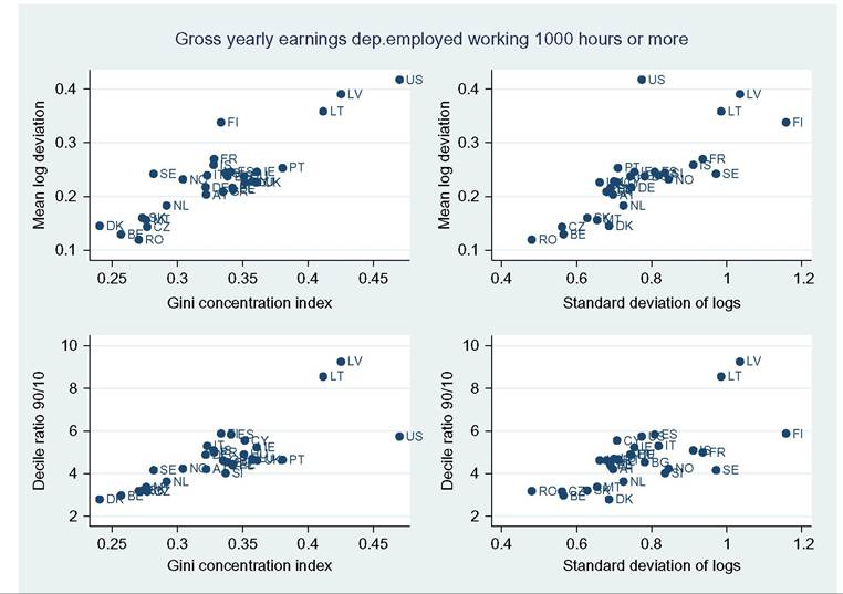
Gini concentration index 1.000 Mean log deviation 0.871 1.000 Standard deviation of logs 0.409 0.770 1.000 Decile ratio 90/10 0.790 0.855 0.689 1.000
Gini of annual labor earnings (including selfemployed and unemployment benefits) Gini of annual gross earnings (hours > 1000) dependent employment Gini of annual hours worked (positive values) Gini of hourly gross wages dependent employment Correlation of hours and hourly wages Austria 0.376 0.322 0.167 0.325 -0.162 Belgium 0.332 0.257 0.173 0.266 -0.284 Bulgaria 0.422 0.338 0.084 0.318 -0.150 Cyprus 0.392 0.352 0.130 0.350 -0.077 Czech Republic 0.341 0.277 0.095 0.252 -0.124 Denmark 0.278 0.240 0.108 0.228 -0.190 Estonia 0.412 0.342 0.117 0.351 -0.208 Finland 0.361 0.333 0.156 0.340 -0.271 France 0.376 0.328 0.176 0.321 -0.201 Germany 0.420 0.322 0.181 0.307 0.038 Greece 0.485 0.335 0.146 0.338 -0.245 Hungary 0.392 0.351 0.084 0.317 -0.004 Iceland 0.338 0.328 0.172 0.337 -0.196 Ireland 0.448 0.361 0.210 0.374 -0.216 Italy 0.407 0.323 0.135 0.308 -0.230 Latvia 0.494 0.425 0.114 0.401 -0.124 Lithuania 0.494 0.412 0.099 0.403 -0.144 Luxembourg 0.428 0.357 0.166 0.355 -0.145 Malta 0.347 0.276 0.109 0.285 bgcolor=white>-0.156 Netherlands 0.359 0.292 0.174 0.290 -0.123 Norway 0.329 0.304 0.134 0.287 -0.115 Poland 0.464 0.342 0.122 0.354 -0.178 Portugal 0.453 0.380 0.104 0.374 -0.144 Romania 0.419 0.270 0.046 0.271 0.045 Slovak Republic 0.347 0.273 0.082 0.253 -0.084 Slovenia 0.397 0.337 0.073 0.314 -0.102 Spain 0.444 0.341 0.142 0.313 -0.209 Sweden 0.321 0.282 0.139 0.336 -0.295 United 0.466 0.361 0.193 0.371 -0.094 Kingdom United States 0.570 0.470 0.164 0.603 0.036 Average 0.408 0.332 0.133 0.331 -0.145